Contents Link to heading
I. Introduction Link to heading
In this post I want to take a trip down SQL memory lane, or just SQLLane for short. Structured Query Language (SQL) is technology that I have been using in many different forms for years. More recently I use it less than I used to and I want to memorialize some of the most important techniques that I have learend in this blog post. I have written prior posts about SQLite and PostgreSQL, NoSQL and DuckDB. Elsewhere I have used Postgres, Teradata, Snowflake, Impala, HiveQL and SparkSQL. SparkSQL and Apache Spark more generally holds a special place in my heart. Spark has the ability to switch between SQL statements and dataframe operations as well as incorporate arbitrary transformation and actions using Python, Scala or Java which make Spark an incredibly powerful technology.
In this post, I will go over SQL techniques that have been extremely helpful in the past and focus on using DuckDB and Apache Spark with some synthetic data for examples. These techniques are not limited to any SQL dialect and are not introductory techinques or queries; the internet is littered with those. Instead I’ll go over some more intermediate and lesser known techniques that can be used by most SQL dialects. The exact syntax will change between dialects, but the ideas will remain the same.
The main topics I’ll cover are:
- Conditional Statements
- TRIM, LOWER & REGEXP_REPLACE
- CASE WHEN .. THEN … END
- Conditional statements within aggregations
- Window Functions
- RANK, DENSE_RANK & ROW_NUMBER
- QUALIFY
- LEAD & LAG
- Moving averages
- Array Operations
- COLLECT_SET/ARRAY_AGG
- EXPLODE/UNNEST
- Special Types of Joins
- Using a JOIN instead of CASE WHEN
- Broadcast joins in Spark
- Filtering by joining
- ANTI JOINS
I’ll also make a few notes of specifics to Spark that are useful in practice. One thing to note is that I use term SparkSQL for both SQL queries as well as Spark dataframe operations. In general the two APIS have the performance and the Spark dataframe API is exteremely well written with a syntax that mirrors SQL so closely I usually just think of the two as interchangable. To some degree they are, but I have found in a few specific cases using the dataframe API provides advantages that I will call out.
First, I’ll create some fake data and then we can get started!
import duckdb
duckdb.query(open('queries/create_names.sql', 'r').read())
duckdb.query(open('queries/create_employees.sql', 'r').read())
duckdb.query(open('queries/create_timeseries.sql', 'r').read())
duckdb.query(open('queries/create_homesales.sql', 'r').read())
duckdb.query(open('queries/create_regions.sql', 'r').read())
II. Conditional Expressions Link to heading
Conditional expressions are queries that involve actions which are dependent on specified conditions being met. In traditional programming languages these are called “if-else” statements. I’ll start out with simple functions for text that require an if-then statement under-the-hood.
1. TRIM, LOWER, & REGEXP_REPLACE Link to heading
These functions are extremely helpful when it comes to text. The TRIM function removes extra white spaces around text. There are versions which only remove extra spaces on the left side LTRIM and right side RTRIM of the text. The LOWER function converts all text to lowercase (or UPPER if you prefer uppercase). Lastly, regular expressions are extremely helpful in SQL since they are optimized operations for finding patterns in text. One particularly helpful technique is REGEX_REPLACE which searches for text that meets a specified pattern and replaces with specified text with what the user defined. Let’s go through a simple example that uses these techniques.
Say I am searching for all records of “Michael Harmon” in the table shown below:
duckdb.query("SELECT id, name FROM names")
┌───────┬──────────────────────┐
│  ID   │         name         │
│ int32 │       varchar        │
├───────┼──────────────────────┤
│     1 │ Michael Harmon       │
│     2 │ Dr. Michael Harmon   │
│     3 │ mr. michael harmon   │
│     4 │  Michael Harmon      │
│     5 │ David Michael Harmon │
└───────┴──────────────────────┘
I should return expect to get records 1-4. If I write a simple naive query using name = 'Michael Harmon' I would only get the first record as a result:
duckdb.query("SELECT id, name FROM names WHERE name = 'Michael Harmon'")
┌───────┬────────────────┐
│  ID   │      name      │
│ int32 │    varchar     │
├───────┼────────────────┤
│     1 │ Michael Harmon │
└───────┴────────────────┘
Instead I’ll use TRIM(LOWER(name)) to make everything the same case and remove extra-spaces to capture record 4. Now I could try to use a wildcard to capture records 2 and 3,
duckdb.query("SELECT id, name FROM names WHERE TRIM(LOWER(name)) LIKE '%michael harmon'")
┌───────┬──────────────────────┐
│  ID   │         name         │
│ int32 │       varchar        │
├───────┼──────────────────────┤
│     1 │ Michael Harmon       │
│     2 │ Dr. Michael Harmon   │
│     3 │ mr. michael harmon   │
│     4 │  Michael Harmon      │
│     5 │ David Michael Harmon │
└───────┴──────────────────────┘
However, that would be a mistake since it would also capture record 5 which is a false positive! Instead of using a wildcard I can use regular expression to remove Dr. and mr. from the names and replace that text with an empty string. This will have the effect of reducing records 3 and 4 to 'michael harmon' which is what I want:
duckdb.query("""
SELECT
    id,
    name
FROM
    names
WHERE
    TRIM(
        REGEXP_REPLACE(
                LOWER(name),'(mr.|dr.)', ''
             )
        ) = 'michael harmon'
""")
┌───────┬────────────────────┐
│  ID   │        name        │
│ int32 │      varchar       │
├───────┼────────────────────┤
│     1 │ Michael Harmon     │
│     2 │ Dr. Michael Harmon │
│     3 │ mr. michael harmon │
│     4 │  Michael Harmon    │
└───────┴────────────────────┘
Great! Now we can move on to more traditional conditional statements!
2. Conditional Statements Link to heading
In modern programming languages “if-else” statements are pretty common statements. In SQL the equivalent is “CASE WHEN … THEN … ELSE …”. You can enumerate any number of cases and the ELSE statement covers the default case that did not match any of the prior specified ones.
As a simple example let’s say we want to know the number of names that are less than 16 characters in the names table, we could add a new column to the table with this information as shown below:
duckdb.query("""
SELECT
    id,
    name,
    CASE WHEN LENGTH(name) < 16 THEN TRUE
         ELSE FALSE
    END AS less_than_15_chars
FROM
    names
""")
┌───────┬──────────────────────┬────────────────────┐
│  ID   │         name         │ less_than_15_chars │
│ int32 │       varchar        │      boolean       │
├───────┼──────────────────────┼────────────────────┤
│     1 │ Michael Harmon       │ true               │
│     2 │ Dr. Michael Harmon   │ false              │
│     3 │ mr. michael harmon   │ false              │
│     4 │  Michael Harmon      │ true               │
│     5 │ David Michael Harmon │ false              │
└───────┴──────────────────────┴────────────────────┘
You can add more conditions by adding more CASE WHEN .. THEN ... statments without ever needing an ELSE (depending on the SQL dialect), but every CASE WHEN statement must always end with an END clause.
3. Conditional Statements With Aggregations Link to heading
Conditional statements can also be used in conjunction with aggregation functions to create more complex queries. For example, you might want to count the number of names that are shorter than a certain length such as shown below,
duckdb.query("""
SELECT
    SUM(CASE WHEN LENGTH(name) < 16 THEN 1 END) AS count_less_than_15_chars
FROM
    names
""")
┌──────────────────────────┐
│ count_less_than_15_chars │
│          int128          │
├──────────────────────────┤
│                        2 │
└──────────────────────────┘
I’ll go over more complex queries with CASE WHEN statements later in this post.
III. Window Functions Link to heading
Window functions are another extremely important concept in SQL. A window function is a function which uses values from one or multiple rows that are related to one another through a so-called partition to return a value for each row. This is a little abstract so let’s go through an example. Suppose we a company table that lists employes and their salaries by department. The table has employee_name, their department and their salary:
duckdb.query("SELECT employee_id, employee_name, department, salary FROM employees")
┌─────────────┬────────────────┬────────────┬────────┐
│ employee_id │ employee_name  │ department │ salary │
│    int32    │    varchar     │  varchar   │ int32  │
├─────────────┼────────────────┼────────────┼────────┤
│           1 │ Alice Johnson  │ Sales      │ 550000 │
│           2 │ Bob Smith      │ Sales      │ 700000 │
│           3 │ Charlie Brown  │ Sales      │ 320000 │
│           4 │ Diana Prince   │ Sales      │ 620000 │
│           5 │ Ethan Hunt     │ Sales      │ 410000 │
│           6 │ Frank Green    │ Sales      │ 490000 │
│           7 │ Grace Adams    │ Sales      │ 520000 │
│           8 │ Henry King     │ Sales      │ 400000 │
│           9 │ Ivy Walker     │ Sales      │ 540000 │
│          10 │ Jack White     │ Sales      │ 470000 │
│          11 │ Laura Chen     │ Sales      │ 380000 │
│          12 │ Marcus Lee     │ Sales      │ 420000 │
│          13 │ Nina Patel     │ Sales      │ 450000 │
│          14 │ Oliver Stone   │ Operations │  85000 │
│          15 │ Patricia Wells │ Operations │  78000 │
│          16 │ Samuel Turner  │ Operations │  90000 │
│          17 │ Tara Benson    │ Marketing  │  95000 │
│          18 │ Uma Garcia     │ Marketing  │  88000 │
│          19 │ Victor Ramirez │ Marketing  │  92000 │
├─────────────┴────────────────┴────────────┴────────┤
│ 19 rows                                  4 columns │
└────────────────────────────────────────────────────┘
We could find the average salary per deparment with the query,
duckdb.query("""
SELECT
    department,
    AVG(salary) dept_avg_salary
FROM
    employees
GROUP BY 1
""")
┌────────────┬───────────────────┐
│ department │  dept_avg_salary  │
│  varchar   │      double       │
├────────────┼───────────────────┤
│ Marketing  │ 91666.66666666667 │
│ Sales      │ 482307.6923076923 │
│ Operations │ 84333.33333333333 │
└────────────┴───────────────────┘
Great, however, what if we want to assign each employee their average department salary? We could do a nested query where we perform the aggregation and then join on the department, but this is kind of sloppy. Instead we can partition employees by their department and aveage over deparment. This can be achieved with the query below,
duckdb.query("""
SELECT
    employee_id,
    employee_name,
    department,
    salary,
    AVG(salary) OVER(PARTITION BY department) AS dept_avg_salary
FROM
    employees
""")
┌─────────────┬────────────────┬────────────┬────────┬───────────────────┐
│ employee_id │ employee_name  │ department │ salary │  dept_avg_salary  │
│    int32    │    varchar     │  varchar   │ int32  │      double       │
├─────────────┼────────────────┼────────────┼────────┼───────────────────┤
│           1 │ Alice Johnson  │ Sales      │ 550000 │ 482307.6923076923 │
│           2 │ Bob Smith      │ Sales      │ 700000 │ 482307.6923076923 │
│           3 │ Charlie Brown  │ Sales      │ 320000 │ 482307.6923076923 │
│           4 │ Diana Prince   │ Sales      │ 620000 │ 482307.6923076923 │
│           5 │ Ethan Hunt     │ Sales      │ 410000 │ 482307.6923076923 │
│           6 │ Frank Green    │ Sales      │ 490000 │ 482307.6923076923 │
│           7 │ Grace Adams    │ Sales      │ 520000 │ 482307.6923076923 │
│           8 │ Henry King     │ Sales      │ 400000 │ 482307.6923076923 │
│           9 │ Ivy Walker     │ Sales      │ 540000 │ 482307.6923076923 │
│          10 │ Jack White     │ Sales      │ 470000 │ 482307.6923076923 │
│          11 │ Laura Chen     │ Sales      │ 380000 │ 482307.6923076923 │
│          12 │ Marcus Lee     │ Sales      │ 420000 │ 482307.6923076923 │
│          13 │ Nina Patel     │ Sales      │ 450000 │ 482307.6923076923 │
│          14 │ Oliver Stone   │ Operations │  85000 │ 84333.33333333333 │
│          15 │ Patricia Wells │ Operations │  78000 │ 84333.33333333333 │
│          16 │ Samuel Turner  │ Operations │  90000 │ 84333.33333333333 │
│          17 │ Tara Benson    │ Marketing  │  95000 │ 91666.66666666667 │
│          18 │ Uma Garcia     │ Marketing  │  88000 │ 91666.66666666667 │
│          19 │ Victor Ramirez │ Marketing  │  92000 │ 91666.66666666667 │
├─────────────┴────────────────┴────────────┴────────┴───────────────────┤
│ 19 rows                                                      5 columns │
└────────────────────────────────────────────────────────────────────────┘
The PARTITION BY statement defines which group a row belongs to before perfoming an aggregation (in this case average) over the group. It is important to note that window functions do not reduce the number of rows returned. Instead they just add additional column based on calculations over a set of rows.
Interestingly DuckDB returns the results in an order that reflects the partitioning instead of the original ordering!
4. RANK, DENSE_RANK & ROW_NUMBER Link to heading
One of the most common usages for window function is for ranking within a group. For example, say we want to rank each employee within a department based on their salary. We can accomplish this with the query,
duckdb.query("""
SELECT
    employee_id,
    employee_name,
    department,
    salary,
    RANK() OVER(PARTITION BY department ORDER BY salary DESC) AS dept_salary_rank
FROM
    employees
ORDER BY department, dept_salary_rank ASC
""")
┌─────────────┬────────────────┬────────────┬────────┬──────────────────┐
│ employee_id │ employee_name  │ department │ salary │ dept_salary_rank │
│    int32    │    varchar     │  varchar   │ int32  │      int64       │
├─────────────┼────────────────┼────────────┼────────┼──────────────────┤
│          17 │ Tara Benson    │ Marketing  │  95000 │                1 │
│          19 │ Victor Ramirez │ Marketing  │  92000 │                2 │
│          18 │ Uma Garcia     │ Marketing  │  88000 │                3 │
│          16 │ Samuel Turner  │ Operations │  90000 │                1 │
│          14 │ Oliver Stone   │ Operations │  85000 │                2 │
│          15 │ Patricia Wells │ Operations │  78000 │                3 │
│           2 │ Bob Smith      │ Sales      │ 700000 │                1 │
│           4 │ Diana Prince   │ Sales      │ 620000 │                2 │
│           1 │ Alice Johnson  │ Sales      │ 550000 │                3 │
│           9 │ Ivy Walker     │ Sales      │ 540000 │                4 │
│           7 │ Grace Adams    │ Sales      │ 520000 │                5 │
│           6 │ Frank Green    │ Sales      │ 490000 │                6 │
│          10 │ Jack White     │ Sales      │ 470000 │                7 │
│          13 │ Nina Patel     │ Sales      │ 450000 │                8 │
│          12 │ Marcus Lee     │ Sales      │ 420000 │                9 │
│           5 │ Ethan Hunt     │ Sales      │ 410000 │               10 │
│           8 │ Henry King     │ Sales      │ 400000 │               11 │
│          11 │ Laura Chen     │ Sales      │ 380000 │               12 │
│           3 │ Charlie Brown  │ Sales      │ 320000 │               13 │
├─────────────┴────────────────┴────────────┴────────┴──────────────────┤
│ 19 rows                                                     5 columns │
└───────────────────────────────────────────────────────────────────────┘
You can use RANK, DENSE_RANK, and ROW_NUMBER to assign rankings within partitions of your data. The difference between them is how they handle ties. RANK will skip ranks if there are ties, DENSE_RANK won’t skip any ranks, and ROW_NUMBER will assign a unique sequential number to each row, regardless of ties.
One thing to be aware of is in Apache Spark if you apply ranking to dataframe without defining a partitioning such as below,
from pyspark.sql.window import Window
import pyspark.sql.functions as F
from pyspark.sql import SparkSession

spark = SparkSession.builder.appName("DuckDB with Spark").getOrCreate()

employee_df = spark.createDataFrame(
                duckdb.query("SELECT employee_id, employee_name, department, salary FROM employees").to_df()
)
win = Window.orderBy(F.col("salary"))
employee_df.withColumn("ranking", F.row_number().over(win)).show()
+-----------+--------------+----------+------+-------+
|employee_id| employee_name|department|salary|ranking|
+-----------+--------------+----------+------+-------+
|         15|Patricia Wells|Operations| 78000|      1|
|         14|  Oliver Stone|Operations| 85000|      2|
|         18|    Uma Garcia| Marketing| 88000|      3|
|         16| Samuel Turner|Operations| 90000|      4|
|         19|Victor Ramirez| Marketing| 92000|      5|
|         17|   Tara Benson| Marketing| 95000|      6|
|          3| Charlie Brown|     Sales|320000|      7|
|         11|    Laura Chen|     Sales|380000|      8|
|          8|    Henry King|     Sales|400000|      9|
|          5|    Ethan Hunt|     Sales|410000|     10|
|         12|    Marcus Lee|     Sales|420000|     11|
|         13|    Nina Patel|     Sales|450000|     12|
|         10|    Jack White|     Sales|470000|     13|
|          6|   Frank Green|     Sales|490000|     14|
|          7|   Grace Adams|     Sales|520000|     15|
|          9|    Ivy Walker|     Sales|540000|     16|
|          1| Alice Johnson|     Sales|550000|     17|
|          4|  Diana Prince|     Sales|620000|     18|
|          2|     Bob Smith|     Sales|700000|     19|
+-----------+--------------+----------+------+-------+
In this case you will force the entire dataframe to collected to on the Spark driver node to be sorted. If your dataframe VERY big this will cause you to blow out of memory.
5. QUALIFY Link to heading
Qualify is a function to filter a table on the results of a window functions. Say I want the highest paid employee in each department, I find this with the following nested query,
duckdb.query("""
SELECT
    employee_id,
    employee_name,
    department,
    salary
FROM (
    SELECT
        employee_id,
        employee_name,
        department,
        salary,
        RANK() OVER(PARTITION BY department ORDER BY salary DESC) AS dept_salary_rank
    FROM
        employees
    ORDER BY employee_id
) B
WHERE
    B.dept_salary_rank = 1
""")
┌─────────────┬───────────────┬────────────┬────────┐
│ employee_id │ employee_name │ department │ salary │
│    int32    │    varchar    │  varchar   │ int32  │
├─────────────┼───────────────┼────────────┼────────┤
│           2 │ Bob Smith     │ Sales      │ 700000 │
│          16 │ Samuel Turner │ Operations │  90000 │
│          17 │ Tara Benson   │ Marketing  │  95000 │
└─────────────┴───────────────┴────────────┴────────┘
However, instead of having a nested query I can use the QUALIFY statement,
duckdb.query("""
    SELECT
        employee_id,
        employee_name,
        department,
        salary
    FROM
        employees
    QUALIFY RANK() OVER(PARTITION BY department ORDER BY salary DESC) = 1
""")
┌─────────────┬───────────────┬────────────┬────────┐
│ employee_id │ employee_name │ department │ salary │
│    int32    │    varchar    │  varchar   │ int32  │
├─────────────┼───────────────┼────────────┼────────┤
│           2 │ Bob Smith     │ Sales      │ 700000 │
│          16 │ Samuel Turner │ Operations │  90000 │
│          17 │ Tara Benson   │ Marketing  │  95000 │
└─────────────┴───────────────┴────────────┴────────┘
This is similary to the HAVING clause where a filtering condition is placed on the results of an aggregation. Both cases can be solved using a subquery and a WHERE clause. Nested queries can be easier to read, but I prefer explicitly listing columns instead of using a * (PLEASE DONT DO THIS it makes it impossible to tell where columns come from when you have long queries and mutliple joins) and having subqueries on top of this makes very long queries which can be tricky to follow.
With Spark Dataframes this syntax issue is not a big deal since it uses a simple filter condition,
win = Window.partitionBy("department").orderBy(col("salary").desc())

# Apply a window function (e.g., row_number) and create a subquery/CTE equivalent
df = employee_df.withColumn("rank", row_number().over(win))

# Filter the results based on the window function output
df.where("rank <= 1").show()
However, one can also can always turn to Common Table Expressions (CTEs) or VIEWS in SparkSQL, but if you pull out QUALIFY you get automatic street credit. :-)
6. LEAD & LAG Link to heading
Now we can get started with window functions for time sersies data! Window functions are great for calculating running totals, moving averages, and other time-based aggregations. A simple example is finding the value for a cell at the prior time period. For instance say we have the following sales data,
duckdb.query("""
SELECT
    sale_id,
    category,
    sale_date,
    amount
FROM
    sales
""")
┌─────────┬─────────────┬────────────┬────────┐
│ sale_id │  category   │ sale_date  │ amount │
│  int32  │   varchar   │    date    │ int32  │
├─────────┼─────────────┼────────────┼────────┤
│       1 │ Electronics │ 2024-01-15 │   1200 │
│       2 │ Furniture   │ 2024-01-20 │    800 │
│       3 │ Electronics │ 2024-02-10 │   1500 │
│       4 │ Clothing    │ 2024-02-15 │    300 │
│       5 │ Furniture   │ 2024-03-05 │    700 │
│       6 │ Clothing    │ 2024-03-10 │    400 │
│       7 │ Electronics │ 2024-03-15 │   2000 │
│       8 │ Furniture   │ 2024-03-22 │    950 │
│       9 │ Electronics │ 2024-04-02 │   1750 │
│      10 │ Clothing    │ 2024-04-08 │    280 │
│      11 │ Electronics │ 2024-04-18 │   2200 │
│      12 │ Furniture   │ 2024-04-25 │    640 │
│      13 │ Clothing    │ 2024-05-01 │    520 │
│      14 │ Electronics │ 2024-05-12 │   1950 │
│      15 │ Furniture   │ 2024-05-20 │    890 │
│      16 │ Clothing    │ 2024-06-03 │    310 │
│      17 │ Electronics │ 2024-06-10 │   2400 │
│      18 │ Furniture   │ 2024-06-15 │    760 │
│      19 │ Clothing    │ 2024-06-21 │    450 │
│      20 │ Electronics │ 2024-07-05 │   1800 │
├─────────┴─────────────┴────────────┴────────┤
│ 20 rows                           4 columns │
└─────────────────────────────────────────────┘
We can find month-over-month change in sales using the LAG function. For clarity I’ll create a monthly sales table first, notice how I have to extract the YEAR and MONTH and concatenate them into an integer as opposed to a string so there is a natural ordering for the window function:
duckdb.query("""
DROP TABLE IF EXISTS monthly_sales;
CREATE TABLE monthly_sales AS (
SELECT
    category,
    CAST(
        CONCAT(YEAR(sale_date)::VARCHAR, LPAD(MONTH(sale_date)::VARCHAR, 2, '0'))
        AS INTEGER
    ) AS year_month,
    SUM(amount) AS amount
FROM
    sales
GROUP BY 1, 2
)
""")
Now I can find the prior month sales with the LAG function:
duckdb.query("""
SELECT
    category,
    year_month,
    this_month_amount,
    prior_month_amount,
    100 * (this_month_amount - prior_month_amount) / prior_month_amount AS month_over_month_change
FROM (
    SELECT
        category,
        year_month,
        amount AS this_month_amount,
        LAG(amount) OVER(PARTITION BY category ORDER BY year_month ASC) AS prior_month_amount,
    FROM
        monthly_sales
    ORDER BY 1,2 ASC
)
""")
┌─────────────┬────────────┬───────────────────┬────────────────────┬─────────────────────────┐
│  category   │ year_month │ this_month_amount │ prior_month_amount │ month_over_month_change │
│   varchar   │   int32    │      int128       │       int128       │         double          │
├─────────────┼────────────┼───────────────────┼────────────────────┼─────────────────────────┤
│ Clothing    │     202402 │               300 │               NULL │                    NULL │
│ Clothing    │     202403 │               400 │                300 │      33.333333333333336 │
│ Clothing    │     202404 │               280 │                400 │                   -30.0 │
│ Clothing    │     202405 │               520 │                280 │       85.71428571428571 │
│ Clothing    │     202406 │               760 │                520 │       46.15384615384615 │
│ Electronics │     202401 │              1200 │               NULL │                    NULL │
│ Electronics │     202402 │              1500 │               1200 │                    25.0 │
│ Electronics │     202403 │              2000 │               1500 │      33.333333333333336 │
│ Electronics │     202404 │              3950 │               2000 │                    97.5 │
│ Electronics │     202405 │              1950 │               3950 │      -50.63291139240506 │
│ Electronics │     202406 │              2400 │               1950 │      23.076923076923077 │
│ Electronics │     202407 │              1800 │               2400 │                   -25.0 │
│ Furniture   │     202401 │               800 │               NULL │                    NULL │
│ Furniture   │     202403 │              1650 │                800 │                  106.25 │
│ Furniture   │     202404 │               640 │               1650 │      -61.21212121212121 │
│ Furniture   │     202405 │               890 │                640 │                 39.0625 │
│ Furniture   │     202406 │               760 │                890 │     -14.606741573033707 │
├─────────────┴────────────┴───────────────────┴────────────────────┴─────────────────────────┤
│ 17 rows                                                                           5 columns │
└─────────────────────────────────────────────────────────────────────────────────────────────┘
7. Moving Averages Link to heading
The last window function technique I’ll mention that is related to time series data is taking the rolling average or moving average of a value over a window. The window in this case is determined both by the PARTITION BY statement as well as a ROWS BETWEEN statement. For instance, if I wanted to get the rolling 3 month average of sales per category I could say,
duckdb.query("""
SELECT
    category,
    year_month,
    amount,
    AVG(amount) OVER(PARTITION BY category
                    ORDER BY year_month ASC
                    ROWS BETWEEN 2 PRECEDING AND CURRENT ROW) AS three_month_moving_average
FROM
    monthly_sales

""")
┌─────────────┬────────────┬────────┬────────────────────────────┐
│  category   │ year_month │ amount │ three_month_moving_average │
│   varchar   │   int32    │ int128 │           double           │
├─────────────┼────────────┼────────┼────────────────────────────┤
│ Electronics │     202401 │   1200 │                     1200.0 │
│ Electronics │     202402 │   1500 │                     1350.0 │
│ Electronics │     202403 │   2000 │         1566.6666666666667 │
│ Electronics │     202404 │   3950 │         2483.3333333333335 │
│ Electronics │     202405 │   1950 │         2633.3333333333335 │
│ Electronics │     202406 │   2400 │         2766.6666666666665 │
│ Electronics │     202407 │   1800 │                     2050.0 │
│ Furniture   │     202401 │    800 │                      800.0 │
│ Furniture   │     202403 │   1650 │                     1225.0 │
│ Furniture   │     202404 │    640 │                     1030.0 │
│ Furniture   │     202405 │    890 │                     1060.0 │
│ Furniture   │     202406 │    760 │          763.3333333333334 │
│ Clothing    │     202402 │    300 │                      300.0 │
│ Clothing    │     202403 │    400 │                      350.0 │
│ Clothing    │     202404 │    280 │          326.6666666666667 │
│ Clothing    │     202405 │    520 │                      400.0 │
│ Clothing    │     202406 │    760 │                      520.0 │
├─────────────┴────────────┴────────┴────────────────────────────┤
│ 17 rows                                              4 columns │
└────────────────────────────────────────────────────────────────┘
Notice with the 3 month moving average, the first month is the current month amount and second month is the average of the second month and the prior month amount. This is because there are not enough prior months to calculate 3 month the average. Depending on the dialect of SQL you are using the first two months are for each category will be NULL instead.
8. Performance Issues With Multiple Expressions in Apache Spark Link to heading
One thing I’ll mention in Spark is that when using dataframes you could be looking to do a lot of different variations of queries. For instance, we could be looking at multiple different moving averages. One way we could do this is to create a loop over each moving average:
df = spark.createDataFrame(duckdb.query("SELECT category, year_month, amount FROM monthly_sales").to_df())

v1_df = df
for i in range(3,6):
    v1_df = v1_df.withColumn(
        f"{i}_month_moving_average",
        F.avg(F.col("amount")).over(
            Window.partitionBy(F.col("category"))
            .orderBy(F.col("year_month").asc())
            .rowsBetween(i, 0)
        )
    )
This isnt so bad when you have a few iterations in the loop, but if you have many withColumn this can lead to issues with your query plan exploding due to projecions and cause performance issues. The query plan can seen using the .explain method,
v1_df.explain()
== Physical Plan ==
AdaptiveSparkPlan isFinalPlan=false
+- Window [avg(amount#24) windowspecdefinition(category#22, year_month#23L ASC NULLS FIRST, specifiedwindowframe(RowFrame, 3, currentrow$())) AS 3_month_moving_average#25, avg(amount#24) windowspecdefinition(category#22, year_month#23L ASC NULLS FIRST, specifiedwindowframe(RowFrame, 4, currentrow$())) AS 4_month_moving_average#27, avg(amount#24) windowspecdefinition(category#22, year_month#23L ASC NULLS FIRST, specifiedwindowframe(RowFrame, 5, currentrow$())) AS 5_month_moving_average#29], [category#22], [year_month#23L ASC NULLS FIRST]
   +- Sort [category#22 ASC NULLS FIRST, year_month#23L ASC NULLS FIRST], false, 0
      +- Exchange hashpartitioning(category#22, 200), ENSURE_REQUIREMENTS, [plan_id=31]
         +- Scan ExistingRDD[category#22,year_month#23L,amount#24]
With Spark 3.0 they introduced a withColumns method which allows you to efficiently apply multiple queries at once using a dictionary as shown below:
queries_dict = {
    f"{i}_month_moving_average":
            F.avg(F.col("amount")).over(
                Window.partitionBy(F.col("category"))
                      .orderBy(F.col("year_month").asc())
                      .rowsBetween(i, 0))
    for i in range(3,6)
}

v2_df = df.withColumns(queries_dict)
v2_df.explain()
== Physical Plan ==
AdaptiveSparkPlan isFinalPlan=false
+- Window [avg(amount#24) windowspecdefinition(category#22, year_month#23L ASC NULLS FIRST, specifiedwindowframe(RowFrame, 3, currentrow$())) AS 3_month_moving_average#31, avg(amount#24) windowspecdefinition(category#22, year_month#23L ASC NULLS FIRST, specifiedwindowframe(RowFrame, 4, currentrow$())) AS 4_month_moving_average#32, avg(amount#24) windowspecdefinition(category#22, year_month#23L ASC NULLS FIRST, specifiedwindowframe(RowFrame, 5, currentrow$())) AS 5_month_moving_average#33], [category#22], [year_month#23L ASC NULLS FIRST]
   +- Sort [category#22 ASC NULLS FIRST, year_month#23L ASC NULLS FIRST], false, 0
      +- Exchange hashpartitioning(category#22, 200), ENSURE_REQUIREMENTS, [plan_id=42]
         +- Scan ExistingRDD[category#22,year_month#23L,amount#24]
To be honest though, I haven’t really seen the issues with the multiple projections occurring. Even in the above examples the query plans are identical.
IV. Array Operations Link to heading
In my opinon array operations are a pretty niche topic in SQL, however, when you need them they are a lifesaver!! One common way to use arrays is to collect information about an enty.
9. COLLECT_SET/ARRAY_AGG Link to heading
Say for instance we run a real-estate sales business with the following sales data,
duckdb.query("""
SELECT
    employee_name,
    sale_date,
    home_price,
    city
FROM
    home_sales
""")
┌───────────────┬────────────┬────────────┬─────────────┐
│ employee_name │ sale_date  │ home_price │    city     │
│    varchar    │    date    │   int32    │   varchar   │
├───────────────┼────────────┼────────────┼─────────────┤
│ Alice Johnson │ 2024-01-10 │     350000 │ New York    │
│ Bob Smith     │ 2024-01-15 │     450000 │ Los Angeles │
│ Charlie Brown │ 2024-02-05 │     300000 │ Chicago     │
│ Diana Prince  │ 2024-02-20 │     600000 │ Miami       │
│ Ethan Hunt    │ 2024-03-12 │     400000 │ Seattle     │
│ Alice Johnson │ 2024-03-25 │     550000 │ New York    │
│ Bob Smith     │ 2024-04-10 │     700000 │ Los Angeles │
│ Charlie Brown │ 2024-04-18 │     320000 │ Chicago     │
│ Diana Prince  │ 2024-05-05 │     620000 │ Miami       │
│ Ethan Hunt    │ 2024-05-22 │     410000 │ Seattle     │
│ Frank Green   │ 2024-06-01 │     480000 │ Dallas      │
│ Grace Adams   │ 2024-06-15 │     510000 │ Phoenix     │
│ Henry King    │ 2024-07-07 │     390000 │ Denver      │
│ Ivy Walker    │ 2024-07-21 │     530000 │ Atlanta     │
│ Jack White    │ 2024-08-09 │     460000 │ Boston      │
│ Frank Green   │ 2024-08-28 │     490000 │ New York    │
│ Grace Adams   │ 2024-09-14 │     520000 │ Los Angeles │
│ Henry King    │ 2024-10-03 │     400000 │ Denver      │
│ Ivy Walker    │ 2024-10-17 │     540000 │ Atlanta     │
│ Jack White    │ 2024-11-05 │     470000 │ Miami       │
├───────────────┴────────────┴────────────┴─────────────┤
│ 20 rows                                     4 columns │
└───────────────────────────────────────────────────────┘
Say we wanted to know which employees sell homes in more than one city and what those cities are. To get the employees that sell in the more than one city can be accomplished with a simple GROUP BY and COUNT, but to get the cities along with that is a little tricker. A simple technique to accomplish this is to collect each city an employee sells in an array and then only take the arrays with more than one entry. The ARRAY_AGG function allows us to collect the entries in a GROUP BY statement as an array as shown below,
duckdb.query("""
DROP TABLE IF EXISTS employees_with_multiple_cities;
CREATE TABLE employees_with_multiple_cities AS
SELECT
    employee_name,
    ARRAY_AGG(city) AS cities_sold_in
FROM (
    SELECT
        employee_name,
        city
    FROM
        home_sales
    GROUP BY 1,2
) BASE
GROUP BY 1
HAVING LENGTH(cities_sold_in) > 1
""")
duckdb.query("SELECT employee_name, cities_sold_in FROM employees_with_multiple_cities")
┌───────────────┬────────────────────────┐
│ employee_name │     cities_sold_in     │
│    varchar    │       varchar[]        │
├───────────────┼────────────────────────┤
│ Grace Adams   │ [Los Angeles, Phoenix] │
│ Jack White    │ [Boston, Miami]        │
│ Frank Green   │ [Dallas, New York]     │
└───────────────┴────────────────────────┘
Notice I had first get the unique set of employee and cities they sold in by removing duplications in cities. With Spark I dont have to go through the deduplication process as the API has a COLLECT_SET which removes any dupications. This means I can write the query as,
sales_df = spark.createDataFrame(duckdb.query("SELECT employee_name, city FROM home_sales").to_df())

result_df = (sales_df.groupBy("employee_name")
                     .agg(F.collect_set("city").alias("cities_sold_in"))
                     .where(F.size("cities_sold_in") > 1)
)

result_df.show()
+-------------+--------------------+
|employee_name|      cities_sold_in|
+-------------+--------------------+
|  Frank Green|  [New York, Dallas]|
|  Grace Adams|[Los Angeles, Pho...|
|   Jack White|     [Miami, Boston]|
+-------------+--------------------+
Now what if I didnt want to have the cities as a list, but instead enumerated out in each row?
10. EXPLODE/UNEST Link to heading
The explode does just this, it is the inverse of collecting elements in an array! In DuckDB this is called UNNEST. A simple example to see how the UNNEST function works is,
duckdb.query("SELECT UNNEST(ARRAY['A', 'B', 'C']) AS letter")
┌─────────┐
│ letter  │
│ varchar │
├─────────┤
│ A       │
│ B       │
│ C       │
└─────────┘
Now say we want to explode the list of cities in the above results, we can do this with the UNNEST function,
duckdb.query("""
SELECT
    employee_name,
    UNNEST(cities_sold_in) AS city
FROM
    employees_with_multiple_cities
""")
┌───────────────┬─────────────┐
│ employee_name │    city     │
│    varchar    │   varchar   │
├───────────────┼─────────────┤
│ Frank Green   │ New York    │
│ Frank Green   │ Dallas      │
│ Grace Adams   │ Phoenix     │
│ Grace Adams   │ Los Angeles │
│ Jack White    │ Boston      │
│ Jack White    │ Miami       │
└───────────────┴─────────────┘
Notice how the rows that were not exploded are repeated for each value in the list (i.e. twice for each employee). In Spark, this is a simple query as ell,
result_df = (result_df.withColumn("city", F.explode("cities_sold_in"))
                      .select("employee_name", "city"))

result_df.show()
+-------------+-----------+
|employee_name|       city|
+-------------+-----------+
|  Frank Green|   New York|
|  Frank Green|     Dallas|
|  Grace Adams|Los Angeles|
|  Grace Adams|    Phoenix|
|   Jack White|      Miami|
|   Jack White|     Boston|
+-------------+-----------+
This is a simple example, but once you start considering using arrays in your SQL queries the types of things you can do in a few lines grows tremendously!!
V. Special Types Of Joins Link to heading
Now to the last topic which is special joins. In the prior sections I covered how to do things with techniques and in this section, I’ll instead focus how do things more effectively using joins.
11. Using A JOIN Instead Of CASE WHEN Link to heading
The first topic is using a JOIN instead of a CASE WHEN statement when assigning values to a new column in table. For instance, suppose we want to append a new column to the home_sales table called region where we group the following cities,
| Region | Cities |
|---|---|
| Northeast | Boston, New York |
| South | Miami, Atlanta |
| Pacific | Seattle, Los Angeles |
| Southwest | Pheonix, Denver, Dallas |
| Midwest | Chicago |
This can be achieved in SQL using a CASE WHEN statement,
duckdb.query("""
SELECT
    employee_name,
    sale_date,
    home_price,
    city,
    CASE
        WHEN city IN ('Boston', 'New York') THEN 'Northeast'
        WHEN city IN ('Miami', 'Atlanta') THEN 'South'
        WHEN city IN ('Seattle', 'Los Angeles') THEN 'Pacific'
        WHEN city IN ('Phoenix', 'Denver', 'Dallas') THEN 'Southwest'
        WHEN city IN ('Chicago') THEN 'Midwest'
    END AS region
FROM
    home_sales
""")
┌───────────────┬────────────┬────────────┬─────────────┬───────────┐
│ employee_name │ sale_date  │ home_price │    city     │  region   │
│    varchar    │    date    │   int32    │   varchar   │  varchar  │
├───────────────┼────────────┼────────────┼─────────────┼───────────┤
│ Alice Johnson │ 2024-01-10 │     350000 │ New York    │ Northeast │
│ Bob Smith     │ 2024-01-15 │     450000 │ Los Angeles │ Pacific   │
│ Charlie Brown │ 2024-02-05 │     300000 │ Chicago     │ Midwest   │
│ Diana Prince  │ 2024-02-20 │     600000 │ Miami       │ South     │
│ Ethan Hunt    │ 2024-03-12 │     400000 │ Seattle     │ Pacific   │
│ Alice Johnson │ 2024-03-25 │     550000 │ New York    │ Northeast │
│ Bob Smith     │ 2024-04-10 │     700000 │ Los Angeles │ Pacific   │
│ Charlie Brown │ 2024-04-18 │     320000 │ Chicago     │ Midwest   │
│ Diana Prince  │ 2024-05-05 │     620000 │ Miami       │ South     │
│ Ethan Hunt    │ 2024-05-22 │     410000 │ Seattle     │ Pacific   │
│ Frank Green   │ 2024-06-01 │     480000 │ Dallas      │ Southwest │
│ Grace Adams   │ 2024-06-15 │     510000 │ Phoenix     │ Southwest │
│ Henry King    │ 2024-07-07 │     390000 │ Denver      │ Southwest │
│ Ivy Walker    │ 2024-07-21 │     530000 │ Atlanta     │ South     │
│ Jack White    │ 2024-08-09 │     460000 │ Boston      │ Northeast │
│ Frank Green   │ 2024-08-28 │     490000 │ New York    │ Northeast │
│ Grace Adams   │ 2024-09-14 │     520000 │ Los Angeles │ Pacific   │
│ Henry King    │ 2024-10-03 │     400000 │ Denver      │ Southwest │
│ Ivy Walker    │ 2024-10-17 │     540000 │ Atlanta     │ South     │
│ Jack White    │ 2024-11-05 │     470000 │ Miami       │ South     │
├───────────────┴────────────┴────────────┴─────────────┴───────────┤
│ 20 rows                                                 5 columns │
└───────────────────────────────────────────────────────────────────┘
But what happens if we add a new city or region? We would need to go back and change our query or possibly add a default case with an ELSE clause. Instead, we could create a mapping table and use a join to assign the region. To do this we can use the mapping table below,
duckdb.query("""
SELECT
    region,
    city
FROM
    regions
""")
┌───────────┬─────────────┐
│  region   │    city     │
│  varchar  │   varchar   │
├───────────┼─────────────┤
│ Northeast │ New York    │
│ Pacific   │ Los Angeles │
│ Midwest   │ Chicago     │
│ South     │ Miami       │
│ Pacific   │ Seattle     │
│ Southwest │ Dallas      │
│ Southwest │ Phoenix     │
│ Southwest │ Denver      │
│ South     │ Atlanta     │
│ Northeast │ Boston      │
├───────────┴─────────────┤
│ 10 rows       2 columns │
└─────────────────────────┘
Now we can join it to the home_sales table as shown below,
duckdb.query("""
SELECT
    L.employee_name,
    L.sale_date,
    L.home_price,
    L.city,
    R.region
FROM
    home_sales AS L
LEFT JOIN
    regions AS R
ON
    L.city = R.city
""")
┌───────────────┬────────────┬────────────┬─────────────┬───────────┐
│ employee_name │ sale_date  │ home_price │    city     │  region   │
│    varchar    │    date    │   int32    │   varchar   │  varchar  │
├───────────────┼────────────┼────────────┼─────────────┼───────────┤
│ Alice Johnson │ 2024-01-10 │     350000 │ New York    │ Northeast │
│ Bob Smith     │ 2024-01-15 │     450000 │ Los Angeles │ Pacific   │
│ Charlie Brown │ 2024-02-05 │     300000 │ Chicago     │ Midwest   │
│ Diana Prince  │ 2024-02-20 │     600000 │ Miami       │ South     │
│ Ethan Hunt    │ 2024-03-12 │     400000 │ Seattle     │ Pacific   │
│ Alice Johnson │ 2024-03-25 │     550000 │ New York    │ Northeast │
│ Bob Smith     │ 2024-04-10 │     700000 │ Los Angeles │ Pacific   │
│ Charlie Brown │ 2024-04-18 │     320000 │ Chicago     │ Midwest   │
│ Diana Prince  │ 2024-05-05 │     620000 │ Miami       │ South     │
│ Ethan Hunt    │ 2024-05-22 │     410000 │ Seattle     │ Pacific   │
│ Frank Green   │ 2024-06-01 │     480000 │ Dallas      │ Southwest │
│ Grace Adams   │ 2024-06-15 │     510000 │ Phoenix     │ Southwest │
│ Henry King    │ 2024-07-07 │     390000 │ Denver      │ Southwest │
│ Ivy Walker    │ 2024-07-21 │     530000 │ Atlanta     │ South     │
│ Jack White    │ 2024-08-09 │     460000 │ Boston      │ Northeast │
│ Frank Green   │ 2024-08-28 │     490000 │ New York    │ Northeast │
│ Grace Adams   │ 2024-09-14 │     520000 │ Los Angeles │ Pacific   │
│ Henry King    │ 2024-10-03 │     400000 │ Denver      │ Southwest │
│ Ivy Walker    │ 2024-10-17 │     540000 │ Atlanta     │ South     │
│ Jack White    │ 2024-11-05 │     470000 │ Miami       │ South     │
├───────────────┴────────────┴────────────┴─────────────┴───────────┤
│ 20 rows                                                 5 columns │
└───────────────────────────────────────────────────────────────────┘
Often changing the region mapping table is easier and more natural than changing the case when staments.
This case leads us to another issue specific to Spark.
12. Broadcast Join in SparkSQL Link to heading
The broadcast join is an extremely helpful join when joining datasests where one dataset is very large and the other is small. Imagine if we had hundreds of millions or billions of sales (for homes this is realistic), but the region mapping was only 50 rows. Since the large table is distributed over many executors and the smaller table is not this can lead to poor performance since there will be A LOT of data shuffling to make sure the correct join keys exist on the executors perfoming the join. Instead, one can broadcast the smaller table to all the executors and then perform the join. This is depicted below (they use the term “worker” instead of “executor”, but they’re the same),
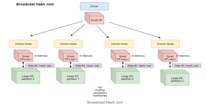
We can accomplish this in code by the following,
regions_df = spark.createDataFrame(duckdb.query("SELECT region, city FROM regions").to_df())

sales_df.join(F.broadcast(regions_df), ["city"], "left").show()
+-----------+-------------+---------+
|       city|employee_name|   region|
+-----------+-------------+---------+
|   New York|Alice Johnson|Northeast|
|Los Angeles|    Bob Smith|  Pacific|
|    Chicago|Charlie Brown|  Midwest|
|      Miami| Diana Prince|    South|
|    Seattle|   Ethan Hunt|  Pacific|
|   New York|Alice Johnson|Northeast|
|Los Angeles|    Bob Smith|  Pacific|
|    Chicago|Charlie Brown|  Midwest|
|      Miami| Diana Prince|    South|
|    Seattle|   Ethan Hunt|  Pacific|
|     Dallas|  Frank Green|Southwest|
|    Phoenix|  Grace Adams|Southwest|
|     Denver|   Henry King|Southwest|
|    Atlanta|   Ivy Walker|    South|
|     Boston|   Jack White|Northeast|
|   New York|  Frank Green|Northeast|
|Los Angeles|  Grace Adams|  Pacific|
|     Denver|   Henry King|Southwest|
|    Atlanta|   Ivy Walker|    South|
|      Miami|   Jack White|    South|
+-----------+-------------+---------+
Note there is a limit to how big a table you can broadcast. You also no longer have to explicitly broadcast the smaller table, Spark can infer this based on your settings! For more information check out the SQL Performance Tuning page on the Spark documentation site.
13. Filtering by Joins Link to heading
This leads us to another good use of joins: using inner joins to filter our data. Suppose we want to find only those sales that occured in the northeast. We could first join the two tables and then filter region = 'Northeast', but this is wasteful since we’ll do a huge join only to remove many of the rows. Instead, we can use the inner join to “filter” out the results we dont want. In the example with home sales, we would first create an inner query to select only cities in the Northeast and then join that to the results table. The query corresponding to this scenario is,
duckdb.query("""
SELECT
    L.employee_name,
    L.sale_date,
    L.home_price,
    L.city,
FROM
    home_sales AS L
JOIN
    (SELECT
        city
    FROM
        regions
    WHERE
        region = 'Northeast'
    ) AS R
ON
    L.city = R.city
""")
┌───────────────┬────────────┬────────────┬──────────┐
│ employee_name │ sale_date  │ home_price │   city   │
│    varchar    │    date    │   int32    │ varchar  │
├───────────────┼────────────┼────────────┼──────────┤
│ Alice Johnson │ 2024-01-10 │     350000 │ New York │
│ Alice Johnson │ 2024-03-25 │     550000 │ New York │
│ Jack White    │ 2024-08-09 │     460000 │ Boston   │
│ Frank Green   │ 2024-08-28 │     490000 │ New York │
└───────────────┴────────────┴────────────┴──────────┘
In many SQL engines the order of when you apply the WHERE clause, i.e. before or after join wont matter as the query optimizer will optimize your query under-the-hood. Spark uses a lazy evaluation model which means that the query optimizer can make these decisions for you when converting your query from the logical plan to the physical plan. For instance, the physical query plan for having the where condition before the join is,
(sales_df.join(F.broadcast(regions_df.where("region = 'Northeast'")), ["city"], "inner" )
         .explain())
== Physical Plan ==
AdaptiveSparkPlan isFinalPlan=false
+- Project [city#38, employee_name#37, region#137]
   +- BroadcastHashJoin [city#38], [city#138], Inner, BuildRight, false
      :- Filter isnotnull(city#38)
      :  +- Scan ExistingRDD[employee_name#37,city#38]
      +- BroadcastExchange HashedRelationBroadcastMode(List(input[1, string, false]),false), [plan_id=273]
         +- Filter ((isnotnull(region#137) AND (region#137 = Northeast)) AND isnotnull(city#138))
            +- Scan ExistingRDD[region#137,city#138]
will be the same physical query plan as having the WHERE condition after the join,
(sales_df.join(F.broadcast(regions_df), ["city"], "inner").where("region = 'Northeast'")
         .explain())
== Physical Plan ==
AdaptiveSparkPlan isFinalPlan=false
+- Project [city#38, employee_name#37, region#137]
   +- BroadcastHashJoin [city#38], [city#138], Inner, BuildRight, false
      :- Filter isnotnull(city#38)
      :  +- Scan ExistingRDD[employee_name#37,city#38]
      +- BroadcastExchange HashedRelationBroadcastMode(List(input[1, string, false]),false), [plan_id=300]
         +- Filter ((isnotnull(region#137) AND (region#137 = Northeast)) AND isnotnull(city#138))
            +- Scan ExistingRDD[region#137,city#138]
One thing to be careful of with Spark is when using a join to filter your tables you are often using a smaller dataframe for filtering. A broadcast join can be appropriate in this situation, but there is another consideration to make. The overlap in the join keys (i.e. city values) between the small dataframe which was broadcasted and the large dataframe only occurs on a few executors in the distributed dataframe table. This leads to many executors having 0 or very few resulting rows following the join. This scenario can lead to data skew in the resulting dataframe. This reveals itself in downstream operations on the dataframe where many executors complete their work quickly and a few take an extremely long time. This situation can be diagnosed in the Spark UI as shown below,
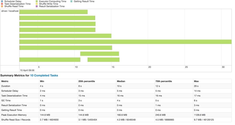
The data skew issue can be corrected by using the coalesce or repartition methods to reduce number of partitions in the dataframe and more evenly distribute the data across the executors. An example is below,
results_df = (sales_df.join(F.broadcast(regions_df), ["city"], "inner").where("region = 'Northeast'")
                      .coalesce(6))

results_df.rdd.getNumPartitions()
6
14. Anti Joins Link to heading
Now to the last topic of this blog post. The anti join is another technique that is not as well known and will garner you street credit when you use it.
Say we to see which real-estate agents have no sales. We can use an ANTI JOIN between the employees and the sales data to do so. An ANTI JOIN will return all records in the left table that have no match in the right table. The syntax in DuckDB is,
duckdb.query("""
SELECT
    L.employee_name,
    L.salary
FROM
    employees L
ANTI JOIN
    home_sales AS R
ON
    L.employee_name = R.employee_name
WHERE
    department = 'Sales' -- I dont want people in marketing or operations
""")
┌───────────────┬────────┐
│ employee_name │ salary │
│    varchar    │ int32  │
├───────────────┼────────┤
│ Marcus Lee    │ 420000 │
│ Nina Patel    │ 450000 │
│ Laura Chen    │ 380000 │
└───────────────┴────────┘
To do this query without an ANTI JOIN we would have to filter on all employees with NULL sales,
duckdb.query("""
SELECT
    L.employee_name,
    L.salary
FROM
    employees L
LEFT JOIN
    home_sales AS R
ON
    L.employee_name = R.employee_name
WHERE
    department = 'Sales' -- I dont want people in marketing or operations
AND
    R.home_price IS NULL
""")
┌───────────────┬────────┐
│ employee_name │ salary │
│    varchar    │ int32  │
├───────────────┼────────┤
│ Marcus Lee    │ 420000 │
│ Nina Patel    │ 450000 │
│ Laura Chen    │ 380000 │
└───────────────┴────────┘
Depending on the problem, you sometimes need to apply the NULL filter in an outer query or else you will inadvertently remove records. In SparkSQL the syntax is the same and the Spark dataframe syntax is,
employee_df.join(sales_df, ["employee_name"], "left_anti").where("department = 'Sales'").show()
+-------------+-----------+----------+------+
|employee_name|employee_id|department|salary|
+-------------+-----------+----------+------+
|   Laura Chen|         11|     Sales|380000|
|   Marcus Lee|         12|     Sales|420000|
|   Nina Patel|         13|     Sales|450000|
+-------------+-----------+----------+------+
VI. Conclusion Link to heading
In this post I covered a few intermediat SQL techniques in DuckDB and PySpark. Many of the techniques are agnostic to the query engine being used, but the syntax might change between SQL engines and dialects. One last resource I will leave you with is the book High Performance Spark. While this book is quite old at this point, it goes over details of Spark that I found very hard to find in any other source. I hope you learned something from this post and hope this post helped you can appreciate the power of Apache Spark, SparkSQL and SQL more generally!