Polars & DuckDB: DataFrames and SQL For Python Without Pandas
2. Getting Set Up On AWS with Docker
4. DuckDB To The Rescue For SQL
Introduction 
In the last few years there has been an explosion of dataframe alternatives to Pandas due to its limitations. Even the original author, Wes McKinney, wrote a blog post about 10 Things I Hate About Pandas.
My biggest complaints about Pandas are:
- High memory usage
- Limited multi-core algorithms
- No ability to execute SQL statements (like SparkSQL & DataFrame)
- No query planning/lazy-execution
- NULL values only exist for floats not ints (this changed in Pandas 1.0+)
- Using strings is inefficient (this too changed in Pandas 1.0+
I should note that many of these issues have been addressed by the Pandas 2.0 release. And while there has been a steady march towards replacing the NumPy backend with Apache Arrow, I still feel the lack of SQL and overall API design is a major weakness of Pandas. Let me expand upon tha last point.
For context I have been using a Apache Spark since 2017 and love it not just from a performance point of view, but I also love how well the API is designed. The syntax makes sense coming from a SQL users perspective. If I want to group by a column and count in SQL or on Spark DataFrame I get what I expect either way: A single column with the count of each item the original dataframes/tables column. In Pandas, this is not the result.
For example using this datas set from NYC Open Data on Motor Vechicle Collisions, I can run a groupby-count expression on a Pandas DataFrame and I get:
import pandas as pd
pd_df = pd.read_csv("https://data.cityofnewyork.us/resource/h9gi-nx95.csv")
pd_df.groupby("borough").count()
Notice this is the number of non nulls in every column. Not exactly what I wanted.
To get what I want I have to use the syntax:
pd_df.groupby("borough").size() # or pd_df.value_counts()
But this returns a Pandas Series. It seems like a trivial difference, but counting duplicates in a column is easy in Spark because we can use method chaining, to the do the equivalent in Pandas I have to convert the series back to a dataframe and reset the index first:
pd_df.groupby("borough").size().to_frame("counts").reset_index().query("counts > 0")
Furthermore, in Pandas there are too many ways to do the same thing. In my opinion, in a well designed API this shouldn't be the case. Lastly, in Pandas, window functions, which are incredibly import in SQL are just awkward to write.
For years I have been using Spark for large datasets, but for smaller ones sticking with Pandas and making do. Recently though, I heard lots of hype about Polars and DuckDB and decide to try them myself and was immediately impressed. In my opinion, Polars is not 100% mature yet, but I still has a lot of potential, many because for me the API is much more similar to Spark's than Pandas is.
In this blog post I go over my first interactions with both libraries and call out things I like and do not like, but first let's get set up to run this notebook on an AWS EC2 instance using Docker.
Getting Set Up On AWS with Docker 
I have mostly used Google Cloud for my prior personal projects, but for this project I wanted to use Amazon Web Services. The first thing I do is create a S3 bucket. I do this from the console by signing on to aws.com and going to the S3 page:
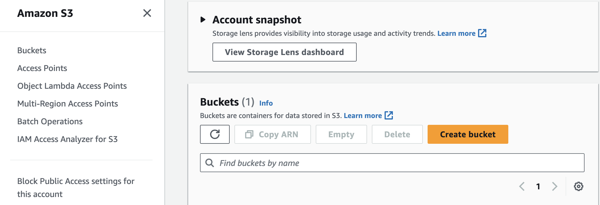
I can click the Create bucket button and create a bucket called harmonskis (for funskis) with all the default settings and click theCreate bucket button on the bottom right side.
Next I need to have access to read and write to and from the S3 bucket so I create an IAM role to do so. Going to the signin dashboard I can search for "IAM" and click on the link. This takes me to another site where selecting the "Roles" link in the the "Access Management" drop down on the left hand side takes me to the following:
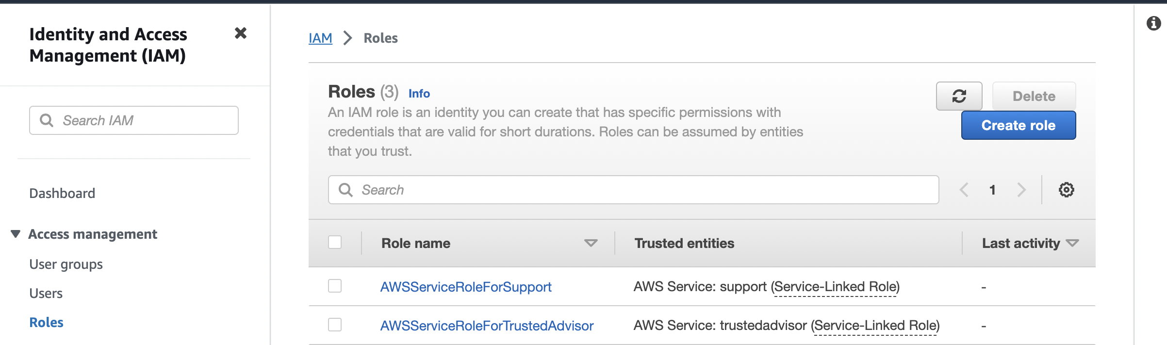
I can click create the Create role button on the top right that takes me to the page:
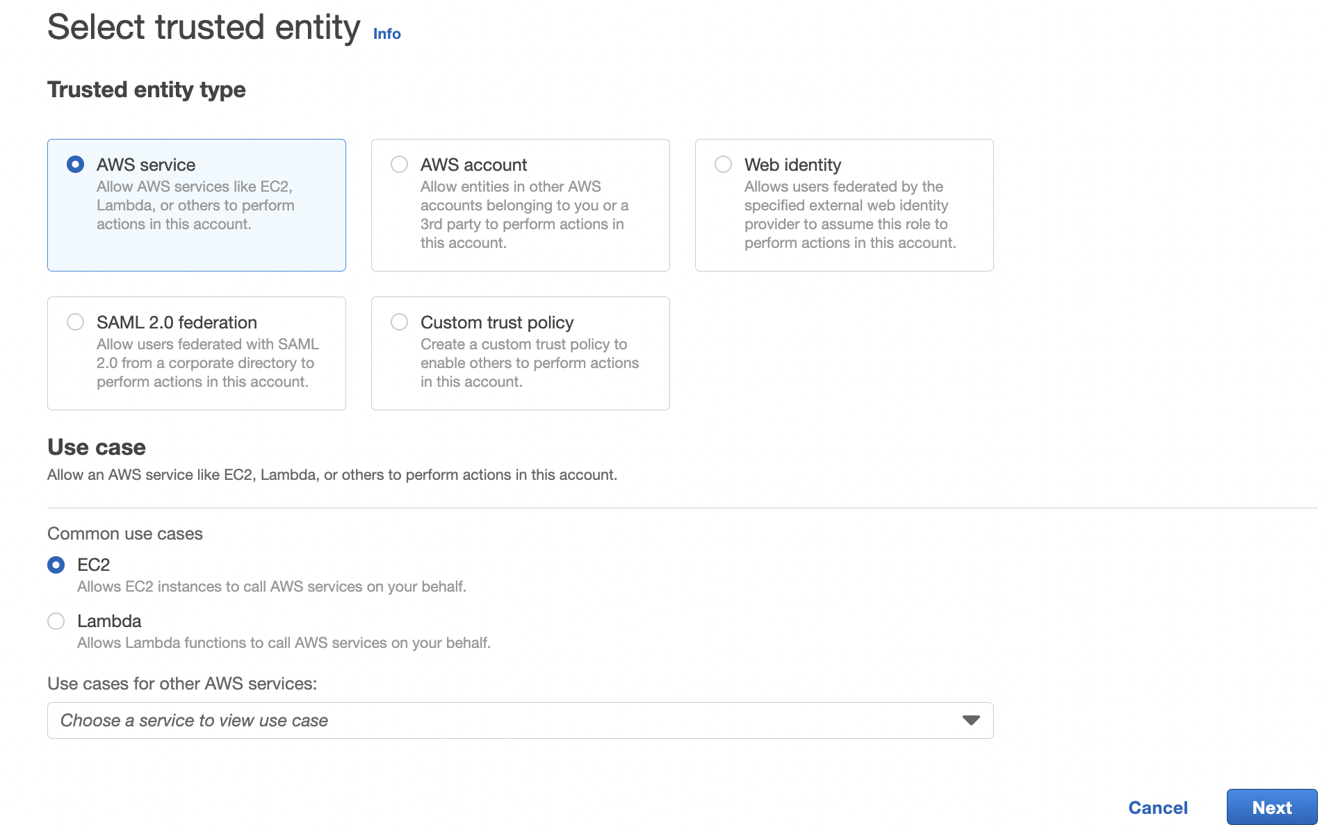
I keep the selection of "AWS Service", select the "ec2" option and then click the Next button on the bottom right. This takes me to a page where I can create a policy. Searching for "s3" I select the following policy that gives me read/write access:
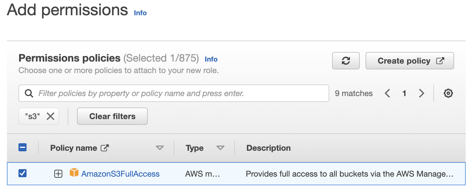
I then click the Next button in the bottom right which takes me to the final page:
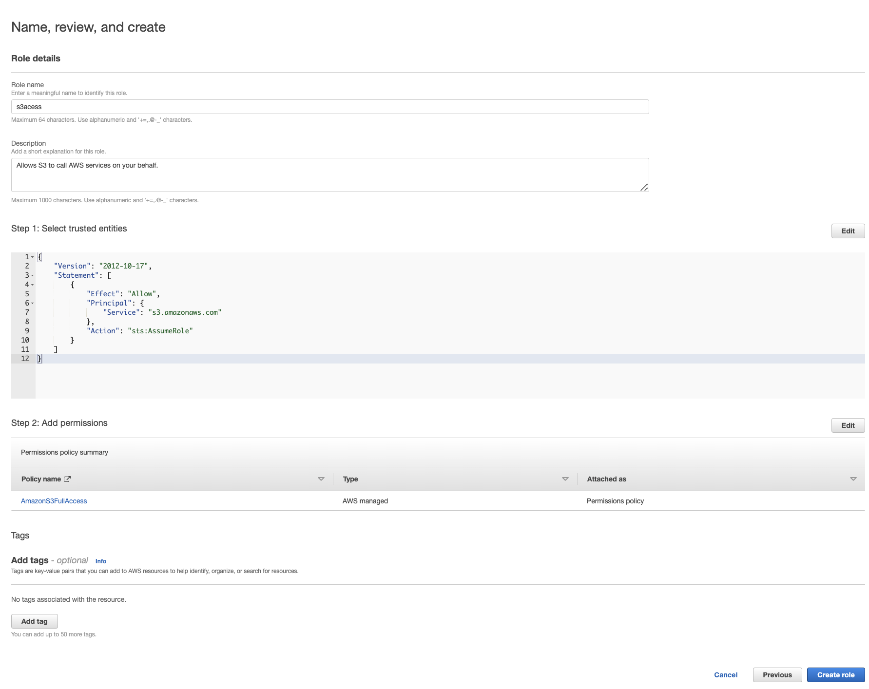
I give the role the name "s3acess" (spelling isnt my best skill) and then click Create role in the bottom right.
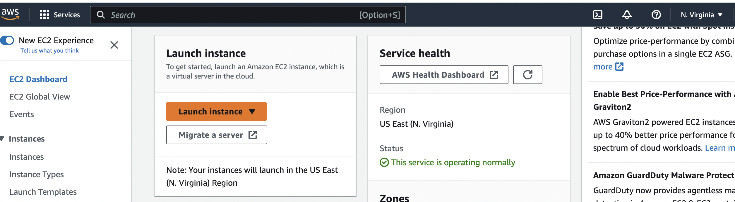
Next I will create my Elastic Compute Cloud
(EC2) Instance instance by going to the console again and clicking on ec2, scrolling down and clicking the orange Launch instance button,
Next I have to make sure I create a keypair file called "mikeskey.pem" that I download.
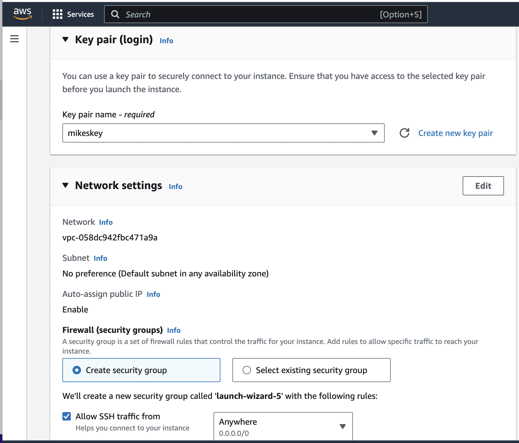
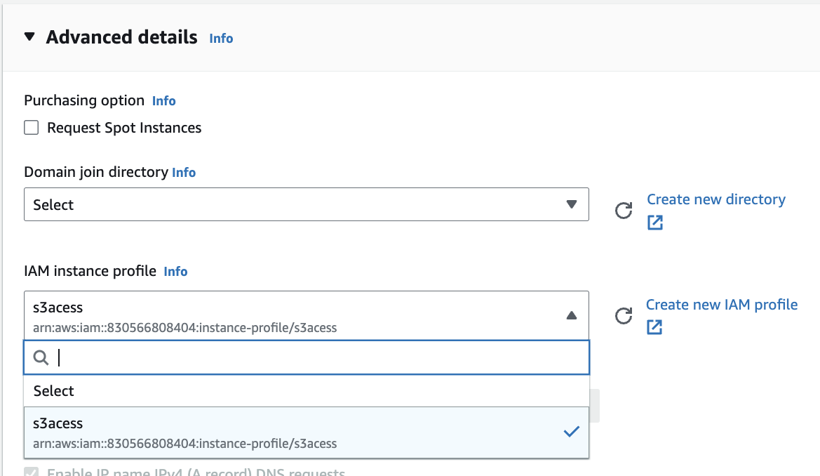
Notice that in the security group I use allows SSH traffic from "Anywhere". Finally, under the "Advanced details" drop down I select "s3acess" (I'm living with my spelling mistake) from the "IAM instance policy":
Once I launch the EC2 instance I can see the instance running and click on Instance ID as shown below:
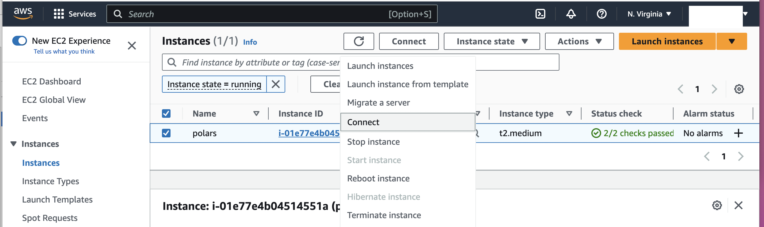
I can then click on the pop up choice of Connect. This takes me to another page where I get the command at the bottom of the page to SSH onto my machine using the keypair I created:
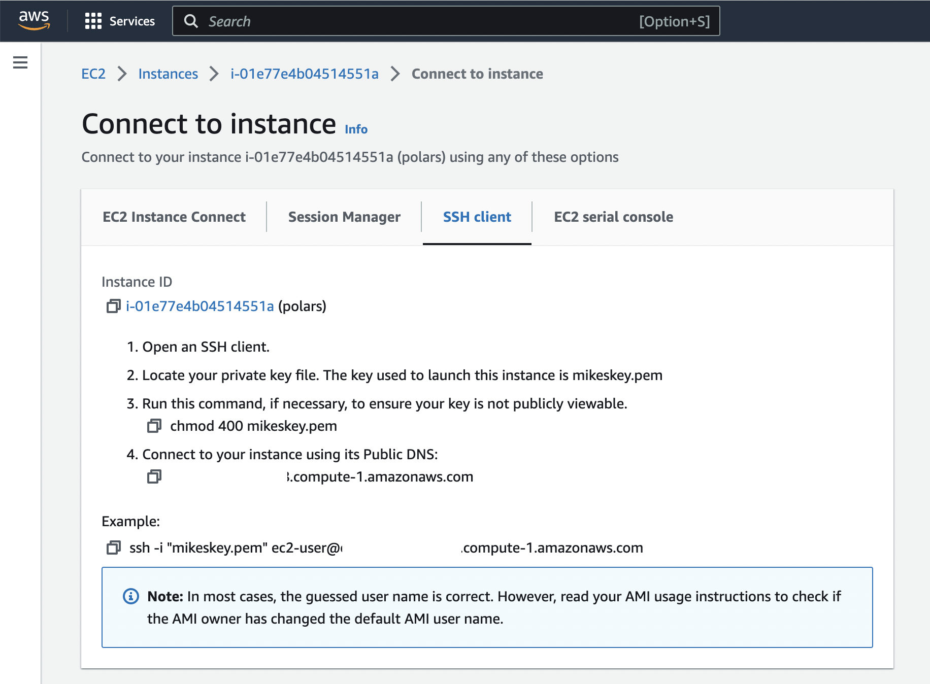
I could ssh onto the server with the following command:
ssh -i <path-to-key>/mikeskey.pem ec2-user@<dns-address>.compute-1.amazonaws.com
Note that I didnt create a user name so it defaulted to ec2-user.
However, since I'll be running jupyter lab on a remote EC2 server I need to set up ssh-tunneling as described here so that I can access it from the web browser on my laptop. I can do this by running the command:
ssh -i <path-to-key>/mikeskey.pem -L 8888:localhost:8888 ec2-user@<dns-address>.compute-1.amazonaws.com
Next I set up git ssh-keys so I could develop on the instance as described here and clone the repo. I can then set up Docker as discussed here. Then I build the image and call it polars_nb:
sudo docker build -t polars_nb .
Finally, I start up the container from this image using port forwarding and loading the current directory as the volume:
sudo docker run -ip 8888:8888 -v `pwd`:/home/jovyan/ -t polars_nb
The terminal shows a link that I can copy and paste into my webbrowser, I make sure to copy the one with the 127 in it and viola it works!
Intro To Polars 
Now that we're set up with a notebook on an EC2 isntance we can start to discuss Polars dataframes. The Polars library is written in Rust with Python bindings. Polars uses multi-core processing making it fast and the authors smartly used Apache Arrow making it efficient for cross-language in-memory dataframes as there is no serialization between the Rust and Python. According to the website the philosophy of Polars is,
The goal of Polars is to provide a lightning fast DataFrame library that:
- Utilizes all available cores on your machine.
- Optimizes queries to reduce unneeded work/memory allocations.
- Handles datasets much larger than your available RAM.
- Has an API that is consistent and predictable.
- Has a strict schema (data-types should be known before running the query).
Let's get started! We can import polars and read in a dataset from NY Open Data on Motor Vehicle Collisions using the read_csv function:
import polars as pl
df = pl.read_csv("https://data.cityofnewyork.us/resource/h9gi-nx95.csv")
df.head(2)
The initial reading of CSVs is the same as Pandas and the head dataframe method returns the top n rows as Pandas does. However, in addition to the printed rows, I also get shape of the dataframe as well as the datatypes of the columns.
I can get the name of columns and their datatypes using the schema method which is similar to Spark:
df.schema
We can see that the datatypes of Polars are built on top of Arrow's datatypes and use Arrow arrays. This is awesome because Arrow is memory efficient and can also used for in-memory dataframes with zero-serialization across languages.
The first command I tried with Polars was looking for duplicates in the dataframe. I found I could do this with the syntax:
test = (df.groupby("collision_id")
           .count()
           .filter(pl.col("count") > 1))

test
Right away from the syntax I was in love.
Then I saw statements returned a dataframe:
type(test)
This is exactly what I want! I don't want a series (even though Polars does have Series data structures). You can even print the dataframes:
print(test)
This turns out to be helpful when you have lazy execution (which I'll go over later). The next thing I tried was to access the column of the dataframe by using the dot operator:
df.crash_date
I was actually happy to see this was not implemented! For me a column in a dataframe should not be accessed this way. The dot operator is meant to access attributes of the class.
Instead we can access the column of the dataframe like a dictionary's key:
df["crash_date"].is_null().any()
The crash dates are strings that I wanted to convert to datetime type (I'm doing this to build up to more complex queries). I can see the format of the string:
df['crash_date'][0] # the .loc method doesnt exist!
To do so, I write two queries:
- The first query extracts the year-month-day and writes it as a string in the format YYYY-MM-DD
- The second query converts the YYYY-MM-DD strings into timestamp objects
For the first query I can extract the year-month-day from the string and assign that to a new column named crash_date_str. Note the syntax to create a new column in Polars is with_columns (similar to withColumn in Spark) and I have to use the col function similar to Spark! I can get the first 10 characters of the string using the vectorized str method similar to Pandas. Finally, I rename the new column crash_data_str using the alias function (again just like Spark). The default for the with_column is to label the new column name the same as the old column name, so we use alias to rename it.
In the second query I use the vectorized string method strptime to convert the crash_date_str column to a PyArrow datetime object and rename that column crash_date (overriding the old column with this name).
These two queries are chained together and the results are shown below.
df = df.with_columns(
            pl.col("crash_date").str.slice(0, length=10).alias("crash_date_str")
      ).with_columns(
            pl.col("crash_date_str").str.strptime(
                pl.Datetime, "%Y-%m-%d", strict=False).alias("crash_date")
)

df.select(["crash_date", "crash_date_str"]).head()
Notice the col function in Polars lets me access derived columns that are not in the original dataframe. In Pandas to do the same operations I would have to use a lambda function within an assign function:
df.assign(crash_date=lambda: df["crash_date_str"].str.strptime(...))
I can see the number of crashes in each borough of NYC with the query
print(df.groupby("borough").count())
There is a borough value of NULL. I can filter this out with the commands:
nn_df = df.filter(pl.col("borough").is_not_null())
Now I can get just the unique values of non-null boroughs with the query:
print(df.filter(pl.col("borough").is_not_null())
        .select("borough")
        .unique())
print(
 df.filter(pl.col("borough").is_not_null())
   .select([
       "borough",
       (pl.col("number_of_persons_injured")  + 1).alias("number_of_persons_injured_plus1")
    ]).head()
)
Doing the same query in Pandas is not as elegant or readable:
(pd_df[~pd_df["borough"].isnull()]
      .assign(number_of_persons_injured_plus1=pd_df["number_of_persons_injured"] + 1)
      [["borough", "number_of_persons_injured_plus1"]]
      .head()
)
To me, the Polars query is so much easier to read. And what's more is that it's actually more efficient. The Pandas dataframe transforms the whole dataset, then subsets the columns to return just two. On the other hand Polars subsets the two columns first and then transforms just those two columns.
Now I can create a Polars dataframe the exact same way as in Pandas:
borough_df = pl.DataFrame({
                "borough": ["BROOKLYN", "BRONX", "MANHATTAN", "STATEN ISLAND", "QUEENS"],
                "population": [2590516, 1379946, 1596273, 2278029, 378977],
                "area":[179.7, 109.2, 58.68, 281.6, 149.0]
})

print(borough_df)
This is the population and area of the boroughs which I got from Wikipedia. I'll save it to s3. It was a little awkward to write to s3 with Polars directly so I'll first convert the dataframe to Pandas and then write to s3:
borough_df.to_pandas().to_parquet("s3://harmonskis/nyc_populations.parquet")
However, reading from s3 is just the same as with Pandas:
borough_df = pl.read_parquet("s3://harmonskis/nyc_populations.parquet")
We'll use it to go over a more complicated query:
Get the total number of injuries per borough then join that result to the borough dataframe to get the injuries by population and finally sort them by borough name.
In Polars this can be using method chaining on the dataframe:
print(
 df.filter(pl.col("borough").is_not_null())
   .select(["borough", "number_of_persons_injured"])
   .groupby("borough")
   .sum()
   .join(borough_df, on=["borough"])
   .select([
       "borough",
       (pl.col("number_of_persons_injured") / pl.col("population")).alias("injuries_per_population")
   ])
   .sort(pl.col("borough"))
)
Doing the same query in the Pandas API would be an awkward mess. As we can see in Polars it's very easy to use method chaining and the resulting syntax reads pretty similar to SQL!
Which brings me to something that was super exciting to see in Polars: sqlcontext. SQLContext in Polars can be used to create a table from a Polars dataframe and then run SQL commands that return another Polars dataframe.
We can see this by creating a table called crashes from the dataframe df:
ctx = pl.SQLContext(crashes=df)
Now I can get the sum of every crash per day in each borough:
daily_df = ctx.execute("""
    SELECT
        borough,
        crash_date AS day,
        SUM(number_of_persons_injured)
    FROM
        crashes
    WHERE
        borough IS NOT NULL
    GROUP BY
        borough, crash_date
    ORDER BY
        borough, day
""")

print(daily_df.collect().head())
Notice I had to use collect() function to get the results. That is because by default SQL in Polars uses lazy execution.
You can see evidence of this when printing the resulting dataframe; it actually prints the query plan:
print(daily_df)
To get back a Polars dataframe from this result I would have to use the eager=True parameter in the execute method.
I can register this new dataframe as a table called daily_crashes in the SQLContext:
ctx = ctx.register("daily_crashes", daily_df)
I can see the tables that are registered using the command:
ctx.tables()
Now say I want to get the current day's number of injured people and the prior days; I could use the lag function in SQL to do so:
ctx.execute("""
    SELECT
        borough,
        day,
        number_of_persons_injured,
        LAG(1,number_of_persons_injured)
            OVER (
            PARTITION BY borough
            ORDER BY day ASC
            ) AS prior_day_injured
FROM
    daily_crashes
ORDER BY
    borough,
    day DESC
""", eager=True)
I finally hit snag in Polars: their doesnt seem to be a lot of support for Window functions. This was initially disappointing since the library was so promising!
Upon further research I found window functions are supported, infact they are VERY WELL supported!. The query I was trying to turns out to be fairly easy to write as dataframe operations using the over expression. This is exactly the same as SQL where the column names within the over(...) operator are the columns you partition by. You can the sort within each partition (or group as they say in Polars) and use shift instead of LAG:
print(
    daily_df.with_columns(
            pl.col("number_of_persons_injured")
              .sort_by("day", descending=False)
              .shift(periods=1)
              .over("borough")
              .alias("prior_day_injured")
).collect().head(8))
It turns out you can do the same thing with Pandas as shown below.
Note that I have to collect the lazy datafame and convert it to Pandas first:
pd_daily_df = daily_df.collect().to_pandas()
pd_daily_df = pd_daily_df.assign(prior_day_injured=
                        pd_daily_df.sort_values(by=['day'], ascending=True)
                          .groupby(['borough'])
                          ['number_of_persons_injured']
                          .shift(1))

pd_daily_df.head(8)
Syntactically, I still perfer the Polars to Pandas.
But let's I really want to use SQL and not do things in the dataframe, atleast to me, it doesnt seem possible with Polars.
Luckily there is another library that support blazingly fast SQL queries and integrates with Polars (and Pandas) directly: DuckDB.
DuckDB To The Rescue For SQL 
I heard about DuckDB when I saw someone star it on github and thought it was "Yet Another SQL Engine". While DuckDB is a SQL engine, it does much more than I thought a SQL engine could!
DuckDB is a parallel query processing library written in C++ and according to their website:
    DuckDB is designed to support analytical query workloads, also known as Online analytical processing (OLAP). These workloads are characterized by complex, relatively long-running queries that process significant portions of the stored dataset, for example aggregations over entire tables or joins between several large tables.
    ...
    DuckDB contains a columnar-vectorized query execution engine, where queries are still interpreted, but a large batch of values (a “vector”) are processed in one operation.
In other words, DuckDB can be used for fast SQL query execution on large datasets. For example the above query that failed in Polars runs perfectly using DuckDB:
import duckdb

query = duckdb.sql("""
    SELECT
        borough,
        day,
        number_of_persons_injured,
        LAG(1, number_of_persons_injured)
            OVER (
                PARTITION BY borough
                ORDER BY day ASC
                ) as prior_day_injured
FROM
    daily_df
ORDER BY
    borough,
    day DESC
LIMIT 5
""")
Now we can see the output of the query:
query
We can return the result as polars dataframe using the pl method:
day_prior_df = query.pl()
print(day_prior_df.head(5))
Now we can see another cool part of DuckDB, you can execute SQL directly on local files!
First we save the daily crash dataframe as Parquet file, but first remember it's a "lazy dataframe":
daily_df
It turns out you cant write lazy dataframes as Parquet using Polars. So first we'll collect it and then write it to parquet:
daily_df.collect().write_parquet("daily_crashes.parquet")
Apache Parquet is a compressed columnar-stored file format that is great for analytical queries. Column-based formats are particularly good for OLAP queries since columns can subsetted and be read in continuously allowing for aggregations to be easily performed on them. The datatypes for each column in Parquet are known which allows the format to be compressed. Since the columns and datatypes are known metadata we can read them in with the following query:
duckdb.sql("SELECT * FROM parquet_schema(daily_crashes.parquet)").pl()
Now we can perform queries on the actualy files without having to resort to dataframes at all:
query = duckdb.sql("""
    SELECT
        borough,
        day,
        number_of_persons_injured,
        SUM(number_of_persons_injured)
            OVER (
                PARTITION BY borough
                ORDER BY day ASC
                ) AS cumulative_injuried
    FROM
        read_parquet(daily_crashes.parquet)
    ORDER BY
        borough,
        day ASC
""")
print(query.pl().head(8))
Pretty cool!!!
Conclusions 
In this post I quickly covered what I view as the limitations of Pandas library. Next I covered how to get set up in with Jupyter lab using Docker on AWS and covered some basics of Polars, DuckDB and how to use the two in combination. The benefits of Polars is that,
- It allows for fast parallel querying on dataframes.
- It uses Apache Arrow for backend datatypes making it memory efficient.
- It has both lazy and eager execution mode.
- It allows for SQL queries directly on dataframes.
- Its API is similar to Spark's API and allows for highly readable queries using method chaining.
I am still new to both libraries, but looking forward to learning more about them.
Hope you enjoyed reading this!