Sentiment Analysis, Part1: ETL With PySpark and MongoDB
Introduction 
I've been itching to learn some more Natural Language Processing and thought I might try my hand at the classic problem of Twitter sentiment analysis. I found labeled twitter data with 1.6 million tweets on the Kaggle website here. While 1.6 million tweets is not substantial amount of data and does not require working with Spark, I wanted to use Spark for ETL as well as modeling since I haven't seen too many examples of how to do so in the context of Sentiment Analysis. In addition, since I was working with text data I thought I would use MongoDB, since it allows for flexible data models and is very easy to use. Luckily Spark and MongoDB work well together and I'll show how to work with both later.
At first I figured I would make this one blog post, but after getting started I realized it was a substaintial amount of material and therefore would break it into two posts. This first post covers the topics of ETL working with Spark and MongoDB. The second post will deal with the actual modeling of sentiment analysis using Spark. The source code for this post can be found here.
ETL With PySpark 
Spark is a parallel processing framework that has become a defactor standard in data engineering for extract-transform-load (ETL) operations. It has a number of features that make it great for working with large data sets including:
- Natural integration with Hadoop for working with large distributed datasets
- Fault tolerance
- Lazy evaluation that allows for behind the scenes optimizations
Spark is also great because allows the one to use a signal framework for working with structured and unstructed data, machine learning, graph computations and even streaming. Some references that I have used for working with Spark in the past include:
The documentation webpage is pretty extensive as well
In this blog post I will NOT be covering the basics of Spark, there are plenty of other resources (like those above) that will do that better than I can. Instead, I want to cover the basics of working with Spark for ETL on text data. I'll explain the steps of ETL I took in detail in this post. While I used a notebook for development, in practice I wrote a Python script that I used to the perform batch analysis. You can find that script here. The script was used to connect to my Atlas MongoDB cluster and I had to change the normalize UDF so that the results are strings instead of arrays of string. This was necessary so that the resulting collection was within the storage limits of the free tier.
Now let's dive into the extract-transform-load operations in Spark and MongodDB!
First we download and extract the dataset from the Kaggle website:
import os
os.system("kaggle datasets download -d kazanova/sentiment140")
os.system("unzip sentiment140.zip")
Next we import the datatypes that we will need for ETL and the functions module from spark.sql
from pyspark.sql.types import (IntegerType, StringType,
                               TimestampType, StructType,
                               StructField, ArrayType,
                               TimestampType)

import pyspark.sql.functions as F
schema = StructType([StructField("target", StringType()),
                   StructField("id", StringType()),
                   StructField("date", StringType()),
                   StructField("flag", StringType()),
                   StructField("user", StringType()),
                   StructField("text", StringType())
                  ])
Now we can define the path to the file, specificy its format, schema and then "read" it in as a Dataframes . Since I am working in standalone mode on my local machine I'll use the address of the csv in my local filsystem:
path = "training.1600000.processed.noemoticon.csv"

# read in the csv as a datafame
df   = spark.read.format("csv")\
                  .schema(schema)\
                  .load(path)
I put read in qoutations since Spark uses a lazy-evaluation model for computation. This means that the csv is not actually read into the worker nodes (see this for definition) until we perform an action on it. An action is any operation that,
writes to disk
brings results back to the driver (see this for definition), i.e. count, show, collect, toPandas,
Even though we have not read in the data, we can still obtain metadata on the dataframe such as its schema:
df.printSchema()
Let's take a look at the first few rows in our dataframe:
df.show(3)
We can see that the table has a target field which is the label of whether the sentiment was positive or negative, an id which is a unique number for the tweet, a date field, a flag field (which we will not use), the user field which is the twitter user's handle and the acual tweet which is labeled as text. We'll have to do transformations on all the fields (except flag which we will drop) in order to get them into the correct format. Specifically, we will:
- Extract relevant fields information the
datefield - Clean and transform the
textfield
Transormations in Spark are computed on worker nodes (computations in Spark occur where the data is in memory/disk which is the worker nodes) and use lazy evaluation. The fact transformations are lazy is a very useful aspect of Spark because we can chain transformations together into Directed Acyclic Graphs (DAG). Because the transformations are lazy, Spark can see the entire pipeline of transformations and optimize the execution of operations in the DAG.
Transform 
We perform most of our transformations on our Spark dataframes in this post by using User Defined Functions or UDFs. UDFs allow us to transform one Spark dataframe into another. UDFs act on one or more columns in a dataframe and return a column vector that we can assign as a new column to our datarame. We'll first show how we define UDFs to extract relevant date-time information from the date field in our dataframe. First let's take a look at the actual date field:
df.select("date").take(2)
Note that we couldnt use the .show(N) method and had to use the .take(N) method. This returns the first N rows in our dataframe as a list of Row objects; we used this method because it allows us to see the entire string in the date field while .show(N) would not.
Our first transformation will take the above strings and return the day of the week associated with the date-time in that string. We write a Python function to do that:
def get_day_of_week(s : str) -> str:
    """
    Converts the string from the tweets to day of week by
    extracting the first three characters from the string.

    """
    day      =  s[:3]
    new_day  = ""

    if day   == "Sun":
        new_day = "Sunday"
    elif day == "Mon":
        new_day = "Monday"
    elif day == "Tue":
        new_day = "Tuesday"
    elif day == "Wed":
        new_day = "Wednesday"
    elif day == "Thu":
        new_day = "Thursday"
    elif day == "Fri":
        new_day = "Friday"
    else:
        new_day = "Saturday"

    return new_day
Next we define the desired transformation on the dataframe using a Spark UDF. UDFs look like wrappers around our Python functions with the format:
UDF_Name = F.udf(python_function, return_type)
Note that specifying the return type is not entirely necessary since Spark can infer this at runtime, however, explicitly delcaring the return type does improve performance by allowing the return type to be known at compile time.
In our case the UDF for the above function becomes:
getDayOfWeekUDF = F.udf(get_day_of_week, StringType())
Now we apply the UDF to columns to our dataframes and the results are appended as a new column to our dataframe. This is efficient since Spark dataframes use column-based storage. In general we would write the transformation as:
df = df.withColumn("output_col", UDF_Name(df["input_col"]) )
With the above UDF our example becomes:
df = df.withColumn("day_of_week", getDayOfWeekUDF(df["date"]))
We can now see the results of this transformation:
df.select(["date","day_of_week"]).show(3)
Another way to define UDFs is by defining them on Lambda functions. An example is shown below:
dateToArrayUDF = F.udf(lambda s : s.split(" "), ArrayType(StringType()))
This UDF takes the date field which is a string and splits the string into an array using white space as the delimiter. This was the easiest way I could think of to get the month, year, day and time information from the string in the date field. Notice that while the return type of the Python function is a simple list, in Spark we have to be more specific and declare the return type to be an array of strings.
We can define a new dataframe which is result of appending this new array column:
df2 = df.withColumn("date_array", dateToArrayUDF(df["date"]))
We can see the result of this transformation below by using the toPandas() function to help with the formatting
df2.select(["date","date_array"])\
   .limit(2)\
   .toPandas()
One other thing to note is that Spark Dataframes are based on Resiliant Distributed Dasesets (RDDs) which are immutable, distributed Java objects. It is perferred when using structured data to use dataframes over RDDs since the former has built-in optimizations. The fact RDDs are immutable means that Dataframes are immutable. While we can still call the resulting dataframe from transformations the same variable name df, the new dataframe is actually pointing to a completely new object under-the-hood. Many times it is desirable to call the resulting dataframes by the same name, but sometimes we have to give the new dataframe a different variable name like we did in the previous cell. We do this for convenience sometimes and othertimes because we do not want to violate the acyclic nature of DAGS.
Next let's define a more few functions to extract the day, month, year, time and create a timestamp for the tweet. The functions will take as an input the date_array column. That is they take as input the array of strings that results from the delimiting of the date field by whitespace. We don't show how these functions are defined (see source code), but rather import them from ETL.src:
from ETL.src.date_utility_functions import (get_month,
                                            get_year,
                                            get_day,
                                            create_timestamp)
Now we create UDFs around these functions as well as creating them around lambda functions to change the target field form 0 to 1:
getYearUDF      = F.udf(get_year, IntegerType())

getDayUDF       = F.udf(get_day, IntegerType())

getMonthUDF     = F.udf(get_month, IntegerType())

getTimeUDF      = F.udf(lambda a : a[3], StringType())

timestampUDF    = F.udf(create_timestamp, TimestampType())

targetUDF       = F.udf(lambda x: 1 if x == "4" else 0, IntegerType())
Now we apply the above UDFs just as we did before. We can get the month of the tweet from the date_array column by applying the getMonthUDF function with the following:
df2 = df2.withColumn("month", getMonthUDF(F.col("date_array")))
Note that we had to use the notation F.col('input_col') instead of df['input_col']. This is because the column date_array is a derived column from the original dataframe/csv. In order for Spark to be able to act on derived columns we need to use the F.col to access the column instead of using the dataframe name itself.
Now we want to apply multiple different UDFs (getYearUDF, getDayUDF, getTimeUDF) to the same date_array column. We could list these operations all out individually as we did before, but since the input is not changing we can group all the UDFs as well as their output column names into a list,
list_udf  = [getYearUDF, getDayUDF, getTimeUDF]
list_cols = ["year", "day", "time"]
and then iterate through that list applying the UDFS to the single input column,
for udf, output in zip(list_udf, list_cols) :
  df2 = df2.withColumn(output, udf(F.col("date_array")))
Now we want want to store an actual datetime object for the tweet and use the timeStampUDF function to do so. Notice how easy it is use UDFs that have multiple input columns, we just list them out!
# now we create a time stamp of the extracted data
df2 = df2.withColumn("timestamp", timestampUDF(F.col("year"),
                                               F.col("month"),
                                               F.col("day"),
                                               F.col("time")))
Now we have finished getting the date-time information from the date column on our dataframe. We now rename some of the columns and prepare to transform the text data next.
# convert the target to a numeric 0 if negative, 1 if postive
df2 = df2.withColumn("sentiment", targetUDF(df2["target"]))

# Drop the columns we no longer care about
df3 = df2.drop("flag","date","date_array", "time", "target")

# rename the tweet id as _id which is the unique identifier in MongoDB
df3 = df3.withColumnRenamed("id", "_id")

# rename the text as tweet so we can write a text index without confusion
df3 = df3.withColumnRenamed("text", "tweet")
We can take a look at our dataframes entries by running,
df3.limit(2).toPandas()
In order to clean the text data we first tokenize our strings. This means we create an array from the text where each entry in the array is an element in the string that was sperated by white space. For example, the sentence,
"Hello my name is Mike"
becomes,
["Hello", "my", "name", "is", "Mike"]
The reason we need to tokenize is two part. The first reason is because we want to build up arrays of tokens to use in our bag-of-words model. The second reason is because it allows us to apply regular-expressions to individual words/tokens and gives us a finer granularity on cleaning our text.
We use the Tokenizer class in Spark to create a new column of arrays of tokens:
from pyspark.ml.feature import Tokenizer

# use PySparks build in tokenizer to tokenize tweets
tokenizer = Tokenizer(inputCol  = "tweet",
                      outputCol = "token")

df4 = tokenizer.transform(df3)
We can take a look at the results again:
df4.limit(2).toPandas()
Now we want to clean up the tweets. This means we want to remove any web addresses, call outs and hashtags. We do this by defining a Python function that takes in a list of tokens and performs regular expressions on each token to remove the unwanted characters and returns the list of clean tokens:
import re

def removeRegex(tokens: list) -> list:
    """
    Removes hashtags, call outs and web addresses from tokens.
    """
    expr    = '(@[A-Za-z0-a9_]+)|(#[A-Za-z0-9_]+)|'+\
              '(https?://[^\s<>"]+|www\.[^\s<>"]+)'

    regex   = re.compile(expr)

    cleaned = [t for t in tokens if not(regex.search(t)) if len(t) > 0]

    return list(filter(None, cleaned))
Now we write a UDF around this function:
removeWEBUDF = F.udf(removeRegex, ArrayType(StringType()))
Next we define our last function which removes any non-english characters from the tokens and wrap it in a Spark UDF just as we did above.
def normalize(tokens : list) -> list:
    """
    Removes non-english characters and returns lower case versions of words.
    """
    subbed   = [re.sub("[^a-zA-Z]+", "", s).lower() for s in tokens]

    filtered = filter(None, subbed)

    return list(filtered)


normalizeUDF = F.udf(normalize, ArrayType(StringType()))
Now we apply our UDFs and remove any tweets that after cleaning result in an empty array of tokens.
# remove hashtags, call outs and web addresses
df4 = df4.withColumn("tokens_re", removeWEBUDF(df4["token"]))

# remove non english characters
df4 = df4.withColumn("tokens_clean", normalizeUDF(df4["tokens_re"]))

# rename columns
df5 = df4.drop("token","tokens_re")
df5 = df5.withColumnRenamed("tokens_clean", "tokens")\

# remove tweets where the tokens array is empty, i.e. where it was just
# a hashtag, callout, numbers, web adress etc.
df6 = df5.where(F.size(F.col("tokens")) > 0)
Looking at the results:
df6.limit(2).toPandas()
LOAD 
Now come to the last stage in ETL, i.e. the stage where we write the data into our database. Spark and MongoDB work well together and writing the dataframe to a collection is as easy as declaring the format and passing in the names of the database and collection you want to write to:
db_name          = "db_twitter"
collection_name  = "tweets"

# write the dataframe to the specified database and collection
df6.write.format("com.mongodb.spark.sql.DefaultSource")\
       .option("database", db_name)\
       .option("collection", collection_name)\
       .mode("overwrite")\
       .save()
That's it for the section on ETL with Spark. Let's take a look at workinng with our MongoDB database next!
MongoDB & PyMongo 
MongoDB is a document based NoSQL database that is fast, easy to use and allows for flexible schemas. I used MongoDB in this blog post since it is document based and is perfect for working inconsistent text data like tweets.
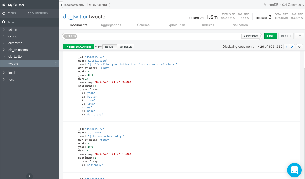
Each database in MongoDB contains collections, each collection contains a set of documents that are stored as JSON objects. In our current example each tweet is a document in our tweets collection in the db_twitter database. MongoDB has nice GUI called Compass. An example view of our tweets collection using Compass is shown below:
Compass gives a nice interface to our database and allows us to run interactive queries on collections and displays easy to read results. One of the most useful features is the ability to analyze your schema. as shown below:
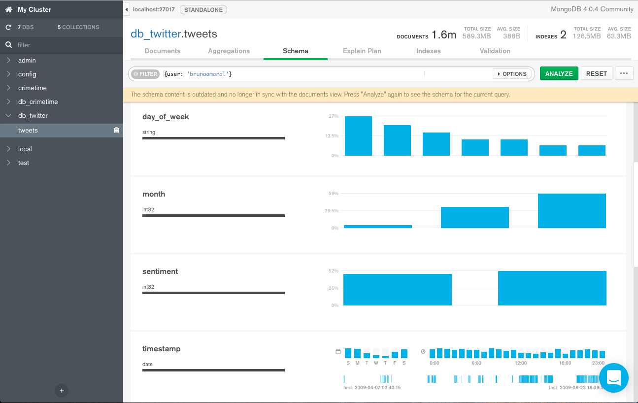
This utility samples our collection to determine the datatypes and values of the fields in your documents. The ability to discern datatypes is especially useful for this type of NoSQL database because fields can have multiple different datatypes. This is in contrast to traditional SQL databases where the entries in tables must rigidly adhere to the defined datatype of that field.
Besides, interacting with a MongoDB database through Compass one can instead use the Mongo Shell, however we will not go over in this feature in this post (except for using it to create an index). Instead we'll use the PyMongo driver which allows us to connect to our Mongo server using Python.
First we import the PyMongo module:
import pymongo
Then we can connect to our Mongo server and db_twitter database:
# connect to the mongo
conn = pymongo.MongoClient('mongodb://localhost:27017')

# connect to the twitter database
db = conn.db_twitter
We can now get the tweets collections with the following:
tweets = db.tweets
Mongo uses JavaScript as it's query language so our queries input and outputs are JSON. In Python we will use dictionaries as the equivalent to JSON. We can run a first example query below:
query = {"day_of_week": "Monday"}
This is a simple filter query where we scan tweets collection and only return documents that occured on Monday,
results = tweets.find(query)
The returned results variable is an interator of documents (a cursor in Mongo terminology). We can iterate through the first 3 documents/tweets with the following:
for res in results.limit(2):
    print("Document = {}\n".format(res))
The _id field is the unique identifier for a document and has been set to the tweet id in this case. As you can see the resulting documents contain all the fields, if instead we wanted only a subset of the fields we can use a projection. Projections list fields to show with the name followed by a 1 and the those not to show with their name followed by a 0:
projection = {"_id":0, "user":1, "tweet":1}

# use the same query as before, but with a projection operator as second arguemtn
results = tweets.find(query, projection)

# print first three results again
for res in results.limit(3):
    print("Document = {}\n".format(res))
With a projection the _id field is shown by default and needs to be explicitly suppressed. All other fields in the document are by default suppressed and need a 1 after them to be displayed.
The filter above was just a simple string matching query. If we wanted to find those tweets that occured on a Monday and in the months before june I would write:
# filter tweets to be on Monday and months before June.
query      = {"day_of_week":"Monday", "month":{"$lt":6}}

# only include the user name, month and text
projection = {"_id":0, "user":1, "month":1, "tweet":1}
results = tweets.find(query, projection)

for res in results.limit(3):
    print("Document = {}\n".format(res))
We can perform a simple aggregation such as finding out the number of tweets that correspond to each sentiment. To do so we use a $group operator in the first line in our query. The field that we group by in this case is the sentiment field:
# Simple groupby example query
count_sentiment = {"$group":
                     {"_id" : {"sentiment":"$sentiment"},  # note use a $ on the field
                      "ct"  : {"$sum":1}
                     }
                  }
The result of this query will be a new document, and this is the reason we need a _id, with the resulting value of the key-value pairs {'sentiment': value} and {'ct': value}. The first key-value pair's value will either be 0 or 1 and the second key-value pair's value will be the number of tweets with that sentiment.
We can then run the query using the aggregate method.
results = tweets.aggregate([count_sentiment], allowDiskUse=True)

for res in results:
    print(res)
First notice that the query is within an array; this allows us to run multiple aggreation queries or 'stages in our aggregation pipeline'. By default each stage in the pipeline can only use 180mb of memory, so inorder to run larger queries we must set allowDiskUse=True to allow the calculations to spill over onto disk.
From this query we can see that, our data set is actually quite well balanced, meaning the number of positive and negative tweets are about the same.
Next we show an example of an aggregation pipeline. The first stage in the pipeline groups the months, and therefore gets the unique months in our dataset:
# get the unique months
get_months = {"$group": {"_id": "$month"} }
The second stage in the pipeline is a projection, which changes the structure of the resulting document:
rename_id  = {"$project":
                      {"_id":0,
                       "month":"$_id"
                    }
             }
In this case the projection operator ($project) suppresses the original _id field for the resulting document of stage one and instead defines the new month key which uses the _id value ($_id operator). We can run this query and see the results:
results = tweets.aggregate([get_months, rename_id])

for res in results:
    print(res)
We can see our Twitter database only has the months: April, May and June. Another example of multiple aggregations is to use the same group-by-count query as above, but filtering first on the month. This dataset only has 3 months of tweets in it and we can use a $match operator to first filter our data to only consider the month of June and then count the number of tweets that occurred in June by using the same query (count_sentiment) as above. The query which performs the match is:
match_query = {"$match": {"month":6}}
We can then run the full pipeline and print the number of tweets that were positive and negative in the month of June:
results = tweets.aggregate([match_query, count_sentiment], allowDiskUse=True)

for res in results:
    print(res)
The last topic I will discuss in the Mongo query langauge is the topic of indexing. Indexing a collection allows for more efficient queries against it. For instance if we wanted to find tweets which occured on a certain date we could write a filter query for it. To execute the query Mongo has to scan the entire collection to find tweets that occured on that day. If we create an index for our tweets collection by the date we create a natrual ordering on the date field. Queries on that field will be much faster since there is now a ordering and entire collection scan is no longer needed. You can have indexes on all sorts of fields, however, your index must be able to fit into memory or else it defeats the purpose of having fast look ups.
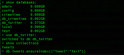
One extremely useful indexing scheme is indexing on the text of the documents in your collection. We can index the tweet field our tweets collection as shown from the Mongo shell below,
Once the index is created you will see:
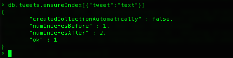
Notice that before creating the above index we actually had one index, but after we have two. The reason is that we have index before indexing our collection is because every collection is by default indexed on the _id field. This also shows us that collections can have multiple indices.
We can now search all our tweets for the phrase "obama" relatively quickly using the query format:
{"$text": {"$search": phrase_to_search}}
We note that the search capabilities ignore stop words, capitilization and punctuation. We show the results below.
search_query = {"$text": {"$search":"obama"} }
projection   = {"_id":0, "user":1, "tweet":1}

# sort the results based on the timestamp
results = db.tweets.find(search_query, projection)\
                       .sort('timestamp', pymongo.ASCENDING)

print("Number of tweets with obama is great: ", results.count())
for res in results.limit(2):
    print("Document = {}".format(res) + "\n")
Next Steps 
In this blog post we went over how to perform ETL operations on text data using PySpark and MongoDB. We then showed how one can explore the loaded data in the Mongo database using Compass and PyMongo. Spark is a great platform from doing batch ETL work on both structured and unstructed data. MongoDB is a document based NoSQL database that is fast, easy to use, allows for flexible schemas and perfect for working with text data. PySpark and MongoDB work well together allowing for fast, flexible ETL pipelines on large semi-structured data like those coming from tweets. In the next blog post will be looking into using PySpark to model the sentiment of these tweets using PySpark!